Congcong Guo, Guicheng Zhang, Shan Jian, Wei Ma, Jun Sun. The impacts of ambiguity in preparation of 80% sulfuric acid solution and shaking time control of calibration solution on the determination of transparent exopolymer particles[J]. Acta Oceanologica Sinica, 2023, 42(4): 50-58. doi: 10.1007/s13131-023-2182-x
Citation:
Congcong Guo, Guicheng Zhang, Shan Jian, Wei Ma, Jun Sun. The impacts of ambiguity in preparation of 80% sulfuric acid solution and shaking time control of calibration solution on the determination of transparent exopolymer particles[J]. Acta Oceanologica Sinica, 2023, 42(4): 50-58. doi: 10.1007/s13131-023-2182-x
Congcong Guo, Guicheng Zhang, Shan Jian, Wei Ma, Jun Sun. The impacts of ambiguity in preparation of 80% sulfuric acid solution and shaking time control of calibration solution on the determination of transparent exopolymer particles[J]. Acta Oceanologica Sinica, 2023, 42(4): 50-58. doi: 10.1007/s13131-023-2182-x
Citation:
Congcong Guo, Guicheng Zhang, Shan Jian, Wei Ma, Jun Sun. The impacts of ambiguity in preparation of 80% sulfuric acid solution and shaking time control of calibration solution on the determination of transparent exopolymer particles[J]. Acta Oceanologica Sinica, 2023, 42(4): 50-58. doi: 10.1007/s13131-023-2182-x
The impacts of ambiguity in preparation of 80% sulfuric acid solution and shaking time control of calibration solution on the determination of transparent exopolymer particles
Institute of Marine Science and Technology, Shandong University, Qingdao 266237, China
2.
Institute for Advanced Marine Research, China University of Geosciences, Guangzhou 511462, China
3.
Research Centre for Indian Ocean Ecosystem, Tianjin University of Science and Technology, Tianjin 300457, China
4.
Huaihe River Basin Eco-environment Monitoring and Scientific Research Center, Huaihe River Basin Eco-environment Supervision and Administration Bureau, Bengbu 233001, China
Funds:
The National Key Research and Development Project of China under contract No. 2019YFC1407805; the National Natural Science Foundation of China under contract Nos 41876134, 41676112 and 41276124; the Tianjin 131 Innovation Team Program under contract No. 20180314; the Changjiang Scholar Program of Chinese Ministry of Education under contract No. T2014253.
The quantification of transparent exopolymer particles (TEP) by colorimetric method is of large error and low repeatability, one major reason of which is related to the absence of clear definition and evaluation for part steps of the original method. It is obscure that the 80% sulfuric acid solution, acted as the extraction solution in the determination of TEP, is prepared based on a volume ratio or mass ratio. Furthermore, the change of solubility of recently available Gum Xanthan (GX) from the market means that the original protocol is no longer applicable, and the grinding of GX stock solution with a tissue grinder is replaced by shaking with a rotating shaker in the study to prevent the excessive dissolution of GX. We found that different preparation techniques could result in the varied concentrations of 80% H2SO4. The duration of shaking during the preparation of standard solution significantly affected the slope of the calibration curve, which caused different correction results of TEP. The impacts of different extraction solution concentrations and shaking time of GX solution on the quantification of TEP were investigated based on the field sampling and laboratory analysis. The extraction capacities of H2SO4 with different concentrations for Alcian Blue were distinct, but had limited effect on the final measuring result of TEP. The change of the standard curve slope came along with the variation of shaking time, which markedly altered the detection limit and calibration result, and the extended shaking time was in favor of the determination of low-concentration TEP. It was suggested that the extraction solution concentration, shaking time and filtration volume of standard solution are required to be well controlled and selected to obtain more accurate results for TEP with different concentrations.
Transparent exopolymer particles (TEP), a class of intermediate between dissolved matter and particulate matter, possess unique physical and chemical properties that can significantly affect the surrounding biological and environmental states (Alldredge et al., 1993; Kiørboe and Hansen, 1993; Myklestad, 1995). TEP are mainly secreted by aquatic microorganisms, including phytoplankton and bacteria (Passow and Alldredge, 1994; Costerton, 1995; Zhou et al., 1998). Diatoms, in particular, continuously release large amounts of extracellular polysaccharides throughout their growth cycle (Hoagland et al., 1993; Krembs et al., 2002; Passow, 2002a). Alternatively, the spontaneous aggregation of these acidic polysaccharides, known as the abiotic assemblage, finally produces TEP whose size is in a range from tens to hundreds of micrometers (Passow, 2000, 2002b). TEP have an independent particle form, instead of covering the surface of cells or being dissolved. The particularity of TEP lies in the nature of the aggregation and the ability to be filtered and collected, and ubiquity in the whole marine system (Alldredge et al., 1993; Passow, 2002b). Previous studies generally believed that the aggregation effect of TEP led to the deposition of a large number of particulate organic carbon and significantly affected the carbon flux to the seabed (Boyd and Newton, 1999; Engel and Schartau, 1999; Radić et al., 2005). However, TEP can suspend and even move towards the surface of seawater, which leads to a continuous accumulation in the surface microlayer, thus having a significant impact on the carbon flux in the surface of oceans (Azetsu-Scott and Passow, 2004; Wurl et al., 2009, 2011). Hence, effects of TEP on marine ecology, biological pump and carbon cycle are of significant spatiotemporal diversity.
TEP are difficult to quantify due to their transparent and shapeless characteristics. The current measurement methods are semi-quantitative in nature (Discart et al., 2015). The first method, microscope counting, is proposed by Alldredge et al. (1993). TEP are prepared by passing a specified volume of seawater onto a 0.4 μm polycarbonate filter, and then stained by Alcian Blue (AB), which makes TEP visible by light microscopy. After that, manual or semi-automatic image analysis is applied for the enumeration of TEP abundance and particle size measurement. The colorimetric method, initially proposed by Passow and Alldredge (1995b), is the most widely used TEP quantitative method at present. The dyed filter is soaked in 80% sulfuric acid solution for 2 h, and then the absorption of supernatant is measured at 787 nm wavelength. Furthermore, the absorption is not available until it was calibrated by the Gum Xanthan (GX). The method of paramagnetic functionalized microspheres is proposed by Mari and Dam (2004), which is based on the adhesion of paramagnetic microspheres to TEP to magnetize and selectively concentrate TEP. The method is isolated from the solution system that is used by the former two means, and the dyeing procedure is eliminated.
Although the colorimetric method is the most commonly used, the shortcomings of which are conspicuous, mainly including interference caused by intracellular material staining, low measuring accuracy and efficiency, poor repeatability of the calibration curve (Discart et al., 2015). In the last decade, parts of the procedures have been modified and improved by later studies to make this technique more reliable (Hung et al., 2003; Thornton et al., 2007; Villacorte et al., 2009). A number of new assistive methods are also being developed, including fluorescent labeling (Fukao et al., 2009; Berman and Parparova, 2010) and introduction of high-precision measuring instruments (Orellana et al., 2011; Verdugo, 2012), but simultaneously, measure time and operation cost have increased.
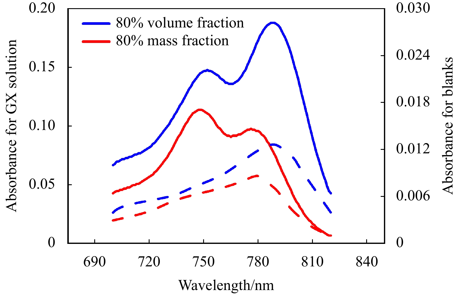
The 80% sulfuric acid solution is conventionally suggested to extract AB from its binding sites with the particulate fraction for the colorimetric method (Passow and Alldredge, 1995b). However, there is no clear definition of the 80% solution. To be specific, there is no foundation in the published papers to confirm that it means a volume ratio or mass ratio between the stock solution and water (Passow and Alldredge, 1995b; Corzo et al., 2000; Passow, 2000; Wurl et al., 2011; Jennings et al., 2017). In China, the percentage of the commercially available stock solution on the label of the bottle is usually considered as a mass fraction. In other countries, by contrast, it is considered that 80% sulfuric acid solution is the volume of sulfuric acid stock solution (mL) to the volume of water (mL). Therefore, there are differences in the preparation of extraction solutions between countries. In the present study, we observed the variations of the maximum absorption wavelength when we chose a different class of 80% sulfuric acid solution (Fig. 1), which proved that the change of extracting solution concentration potentially affected the measurement accuracy and result. As previously reported by Passow and Alldredge (1995b), the maximum absorption of AB extracted by sulfuric acid solution with a volume fraction of 80% lies at 787 nm. The maximum absorption, by contrast, was observed at 748 nm when the concentration of the extraction solution became a mass fraction of 80%. In view of the difference in the understanding of percentage for the stock solution, there may have been inter-nation discrepancies in the protocol of TEP measurement. In addition, during the preparation of a standard solution, it was found that the shaking time had a profound influence on the calibration results. This study is intended to investigate the influences of the two different preparation techniques of extraction solution and shaking time on the standard curves. Based on the TEP samples collected from the eastern Indian Ocean (EIO) in 2019, we further test the variations of extracting effect and calibration results of TEP based on the different protocols. Although it is limited to a few samples and research environment, and the conclusions we gained from this study are initial, the research results are of reference value to control the potential errors and uncertainties of TEP determination.
Figure
1.
The continuous absorption spectrum of Alcian Blue in a sulfuric acid solution of 80% volume fraction (blue) and mass fraction (red), with the absorbance peak being at 787 nm and 748 nm, respectively. Solid lines denoted the absorption for Gum Xanthan (GX) solution dyed with Alcian Blue. Dashed lines denoted the blanks by filtering the same volume of Milli-Q water.
The field investigation was conducted on the R/V Shiyan 3 in EIO from March 20 to June 2, 2019. Water samples for TEP were collected from six stations by a Rosette sample system equipped with a CTD (Conductivity, Temperature and Depth; Model: Seabird 19 Plus) in situ (Fig. 2). Seven water depth samples were collected at each station, i.e., 0 m, 25 m, 50 m, 75 m, 100 m, 150 m, 200 m.
Figure
2.
The distribution of sampling stations in the study area.
Two different concentrations of 80% solutions were prepared based on the volume fraction and mass fraction, respectively. The stock solution (analytically pure) that is purchased from the market is commonly not 100% sulfuric acid. In the study, the stock solution comes at 98%. If it is considered as a volume fraction, then the calculation to make 100 mL of a 80% solution from a 98% stock is
It means to mix 81.6 mL of 98% stock into 18.4 mL water to make a 80% solution. However, it is different when the percentage of the stock solution is thought to be a mass fraction. The density of the stock is estimated as 1.84 g/cm3 and the density of water is 1 g/cm3. Assuming that V (mL) of the stock is needed to make 100 mL of a 80% solution, then the formula is
In consequence, we need to mix 68.9 mL of the stock into 31.1 mL of water to make a 100 mL solution with 80% mass fraction, which is equal to 67.5% volume fraction.
2.3
Analytical methods of TEP
Discrete seawater samples (volume: 300−400 mL) for TEP were filtered in 6 replicates through 0.4 μm pore-size polycarbonate filter by the polysulfone filtration apparatus at <100 mm Hg onboard, after which the particles on the filter were stained for <5 s with 0.5 mL of a 0.02% aqueous solution of AB in 0.06% acetic acid at pH 2.5. Excess dye was fully rinsed with Milli-Q water. As a blank control, equivoluminal Milli-Q water like the treatment group was filtered in triplicates onto filters and then stained with the same procedures described above. Stained filters were then preserved at low temperature (−20℃) without light. After returning back to the laboratory, the prepared filters were put in precleaned 20 mL glass scintillation vials with polypropylene screw caps. The samples were divided into two groups, including the volume fraction group and the mass fraction group, each of which was extracted by adding 6 mL 80% H2SO4 calculated by the volume and mass fraction, respectively. It is essential to seal the glass vials with caps during extraction for 2 h considered the highly hygroscopic nature of sulfuric acid and shake manually 3−5 times for the sufficient dissolution. Each individual group was in triplicates. The absorption of the extraction solution of each group was recorded at 787 nm (volume fraction group) or 748 nm (mass fraction group) using a spectrophotometer (UV-2300). All related plastic and glassware were previously cleaned with 2% HCl solution overnight and then rinsed at least five times with Milli-Q water.
2.4
Calibration procedure
Calibration was indispensable because AB shows evident batch variation in both purity and solubility (Passow and Alldredge, 1995b). The stock solution for calibration was performed by mixing 15 mg of GX (Sigma) into 200 mL of Milli-Q water, and then shook by a rotating shaker with a rotational speed of 150−160 r/min for a specific time to evenly break up the gellike particles. In this study, we set two separate shaking time: 0.5 h and 1 h to prepare two types of GX solution with different dissolution capabilities. Dry weights of particles retained on the filters were determined by filtering a series of (0 mL, 0.2 mL, 0.5 mL, 0.8 mL, 1.0 mL, 1.2 mL, 1.5 mL, 2.0 mL, 2.5 mL, 3.0 mL) standard solutions, in six replicates for each type of solution, onto preweighted filters with an analytical balance (Sartorius, MSE3.6P-0CE-DM). After that, the filters were stained according to the protocol mentioned above, and then stained filters were soaked into the two specifications of sulfuric acid for 2 h accompanied by gentle agitations of 3−5 times, respectively. In the end, four different treatment conditions were set up in this experiment: 80% volume fraction and shaking for 0.5 h (T1), 80% mass fraction and shaking for 0.5 h (T2), 80% volume fraction and shaking for 1 h (T3), 80% mass fraction and shaking for 1 h (T4). Triplicate copies were controlled for each treatment condition.
The maximum absorbance of the two kinds of aliquot of sulfuric acid solution was recorded against Milli-Q water to make sure that the photometric characteristics of the two extraction solution batches were consistent and there was no potential artificial contaminant. No significant difference in absorbance was found between the two batches of extraction solution, thus eliminating the interference of background value. The spectrophotometer was then blanked with extraction solution. The absorbance of triplicate blanks that filtered the equivalent volume of Milli-Q water instead of the standard solution was also measured.
The calibration curve was made based on the linear regression of the blank-corrected absorption of stained GX vs. GX dry weight. The calibration factor $ {f}_{x} $, which was used to quantify the concentration of TEP, was calculated as 1/slope of the calibration curve (Passow and Alldredge, 1995b). As there are many factors influencing the process of making the standard curve, the fitted curves are prone to large variations and errors. Therefore, the standard curves of this experiment were obtained after repeating the measurements several times in accordance with the unified procedure when the slope of the standard curve tended to be stable.
2.5
Statistical analysis
Statistical analyses were implemented by SPSS version 25.0 (SPSS Inc., IBM, USA). A T-test was performed to estimate whether the difference was significant between the measurement results of different treatment groups. The map of the station distribution was charted by Ocean Data View 5.1.7. The linear fitting and column charts were made using Origin 8.0.
3.
Results
3.1
Calibration curves
The standard curves of the four treatment groups were presented in Fig. 3. The high R2 closed to 1 proved that the regressions based on the dataset were reliable. We observed standard curves with different slopes between treatments (Table 1). Above all, in the same shaking time, the absorbance of stained XG was significantly affected by different extraction solutions, with the absorption values of Curve1 (C1) or Curve3 (C3) significantly higher than that of Curve2 (C2) or Curve4 (C4) (p<0.01). It was distinct that C1 was visibly steeper than C2 (Fig. 3), which demonstrated the different extraction of the two solutions. More precisely, differences of absorbance between different extraction solutions were not obvious for the calibration points with a low mass of GX (<10 μg), but the situation was different for those points with a high mass of GX (>10 μg). It seemed that the H2SO4 with 80% volume fraction had a higher extracting capability for the substrate in high concentration than the H2SO4 with 80% mass fraction.
Figure
3.
Calibration curves of different treatment groups (Curve1 (C1): calibration curve of T1; Curve2 (C2): calibration curve of T2; Curve3 (C3): calibration curve of T3; Curve4 (C4): calibration curve of T4). Each calibration point denotes the average absorption of the triplicate copies. Solid (empty) points denote shaking time of 0.5 h (1 h). Solid (dashed) lines are fitted by data points of shaking for 0.5 h (1 h). Error bars represent standard deviation. Other relevant information is shown in Table 1.
Furthermore, the slope of calibration curves made with more shaking time (1 h) of GX solution significantly decreased compared to that with less shaking time (0.5 h) as shown in Fig. 3. The effects of shaking time on the calibration points that filtered standard solution with small bulk (<1 mL) were not marked as the recorded absorbances and masses of GX were parallel between treatments with different shaking time (between C1 and C3; C2 and C4). The variations, in comparison, were principally embodied in the points with relatively large filtered bulk (>2 mL). The mass of retained GX shaken for 1 h was evidently less than that shaken for 0.5 h, accompanied by lower absorbances (Fig. 3), which manifested that shaking lasted too long will accelerate the dissolution of GX solute. It suggested that the choice of shaking time should be treated with caution by reason of its prominent impact on the slope of the calibration curve.
3.2
Extraction efficiency and detection limits
The extraction efficiency of sulfuric acid with different concentrations was represented as the relative magnitude of the respective absorbances. It was concluded that more dyed TEP would be extracted out of the filter by a higher concentration of extraction solution, i.e., 80% volume fraction. In addition, for the shaking time of 0.5 h, the extraction efficiency between the two sulfuric acid solutions, which was manifested as the difference of recorded absorbances between C1 and C2, showed a quadratic function of GX mass (Fig. 4), indicating that the differential extraction by the two solutions enhanced dramatically with the rise of available objects (standards or TEP). It is noticeable, however, that the rising tendency was inconspicuous when the mass of GX stained on the filter was less than 12 μg (Fig. 4). Hence, even choosing different concentrations of sulfuric acid solution, the influence on the experimental result is potentially limited in the low-concentration condition.
Figure
4.
The change of extraction efficiency difference between T1 and T2 with the Gum Xanthan dry weight.
The protocol to calculate the limit of detection (LOD, in microgramme-GX) of standard curve followed the theory of Corley (2003) and was introduced by Bittar et al. (2018). There was little difference in LOD between the curves with the same shaking time (C1 and C2; C3 and C4). The LOD of the method is a function of the slope and mean-square error (MSE) of the standard curve. Although the calibration curve of C1 possessed a greater slope (0.0042) than that of C2 (0.0028), the calibration points of C2 tended to be of less MSE than the former, which demonstrated that the prediction models described experimental data with better accuracy. The shaking time had a greater effect on the LOD as the curves with longer shaking time tended to be of lower LOD (Table 1). Taken as a whole, the lower LOD comes with the relatively smaller slope and better fitting effect, which are more suitable for the detection of low-concentration TEP.
3.3
Measuring result of TEP
The concentrations of TEP calculated by different standard curves were recorded in Fig. 5. The distribution of TEP was characterized by a high concentration in the surface, subsurface and deep chlorophyll maximum (DCM) layer, while it customarily showed a significant reduction below the DCM layer due to the inhibition of biological activity (Ramaiah et al., 2001; Azetsu-Scott and Passow, 2004; Prieto et al., 2006; Ortega-Retuerta et al., 2009). Hence, the upper layer was regarded as a high concentration area, and the lower layer was considered a low-concentration area. It was noted that different treatment conditions have distinct impacts on the measuring results of TEP with high and low concentrations.
Figure
5.
The distribution of transparent exopolymer particles (TEP) concentrations in the upper (0−75 m) and lower (100−200 m) layers of the water column. a. upper layer; b. lower layer. Each column denotes the average TEP concentration of four or three sampling layers. Error bars represent standard deviation. The asterisks above the columns indicate that the difference of measuring results are significant compared with the group of T1. *, difference is significant at the 0.05 level (2-tailed). **, difference is significant at the 0.01 level (2-tailed). Plus signs above the columns indicate that the results are below the limit of detection.
In order to evaluate the influence of different conditions on the measuring results, the T1 was considered as the control group, and then the measuring results of remaining groups (T2, T3 and T4) and the control group were compared statistically, with the statistical conclusion shown in Fig. 5. For TEP with high concentration (upper layer), no significant difference was observed between T2 and T1 (p>0.05, Fig. 5a), which indicated that the change of extraction solution concentration has no significant impact on the measuring result of the high concentration sample. However, the absorbance extracted by different sulfuric acid solutions was significantly different (p<0.05), according with the absorbance difference between C1 and C2. The results of T3 were significantly higher than those of T1, thus proving that the shaking time during the preparation of GX solution significantly affected the calibration results of TEP. Although half of the measured results in T4 were not significantly different from those in T1, the relative variation between the two treatments was yet large (Fig. 5a). As a consequence, changing the two variables at the same time influenced remarkably the results of determination.
For TEP with low concentration (lower layer), the variations were consistent with those of high concentration TEP (upper layer) except for the particular station (Fig. 5b). The relative variations of determination results between treatments were considerably small since the low-level magnitude of the data. Hence, the focus should be on whether the measurement results are above the LOD for samples with low concentration. It was thus note-worthy that the determination results of the two stations (S10-01, EQ-11) were below the LOD in the group of T1. Actually, at the bottom depth (150−200 m), the TEP concentrations calculated by the slope of C1 or C2 in more than half of the stations were below the LOD, which demonstrated that less shaking time was not conducive to the calibration of low-concentration TEP.
4.
Discussion
The drafting of GX standard curves is well known to be of low repeatability and high linear error, which were attributed to the dyeing ability variation of AB solutions prepared by different batches. However, we plotted standard curves with evidently different slopes using the same batch of AB, and the reasons behind which were numerous. As mentioned above, the variation of sulfuric acid solution concentration caused a differential extraction and affected the slope of the standard curve. It is operationally difficult to obtain well-proportioned and stable GX stock solution. In addition, the blocking effect of filters potentially leads to the disproportionate increase of absorbance when filtering overmuch GX solution. To sum up, we need to take various factors into consideration to optimize the calibration results.
4.1
The impact of different sulfuric acid solution concentrations
In the original protocols, Passow and Alldredge (1995b) had explored various factors that could interfere with the measurement results, including concentration of dye solution, pH, staining time, soaking time of filters in sulfuric acid, filtration pressure, etc., except for the effect of sulfuric acid concentration on the results. In the study, by comparison, we found that different concentrations of sulfuric acid solution have an effect on the peak wavelength and absorbance of standard and TEP (Fig. 3). It is reasonable to speculate that the extraction ability could increase with the concentration of the extraction solution, on account of the absorbance of sulfuric acid solution with 80% volume fraction being higher. Actually, the absorption spectrum showed two significant characteristic peaks with different strength (Fig. 1). However, the two absorbance peaks changed both in the strength and position with the decrease of sulfuric acid solution concentration. More specifically, as shown in Fig. 1, the absorption peaks shifted towards the short wave and significantly weakened, especially for the one at 787 nm. The drastic reduction of the absorption peak at 787 nm indicated the degradation of the characteristic chromophore corresponded to the wavelength. There are more characteristic groups that come with more stained substrates, which also means that more groups could be destroyed during the extracting process. As a result, the differences of absorbances extracted by different concentrations of sulfuric acid solutions, i.e., extraction efficiency as mentioned above, would be increasingly apparent (Fig. 4).
Furthermore, we set up a series of concentration gradients of the sulfuric acid solution to explore the influence of extraction concentration on the absorption peaks (Fig. 6). No evident variation in strength was observed for the absorption peak at 787 nm in the extraction solution of 70%, 75%, 80% and 90%. Meanwhile, the absorption peak of 787 nm increased to a maximum for 95% sulfuric acid solution, while it reached the lowest point for 67.5% (or 80% mass fraction) sulfuric acid solution. This finding can be attributed to the possibility that high concentration of the extraction solution is more conducive to the development of characteristic group. Nevertheless, the strength of the absorption peak at 748 nm enhanced to a high level in 70% and 75% sulfuric acid solution, which proved that the corresponding chromophore of dyes was more stable in the low concentration of a sulfuric acid solution. It seemed that the absorption peak strength of 787 nm was more susceptible to the sulfuric acid solution concentration than that of 748 nm according to Fig. 3, i.e., the corresponding chromophore at 787 nm was more sensitively affected by sulfuric acid solution concentration. The drastic reduction of absorption strength at 787 nm in response to the extraction concentration suggested that a specific chemical process mediated the inhibition of colour developing. The chemical properties of sulfuric acid changed with the concentration, and the chemical reactions as well as the relevant products varied in sulfuric acid solutions of different concentrations, which potentially influenced the measuring result. The chance of incomplete extraction of AB by low concentration of extraction solution, which may happen for high concentration samples, is less likely. The data of Fig. 6 were collected by filtering 1.5 mL GX stock solution according to the above protocol, and that meant less amounts of particles were retained on the filters. In addition, the blank that only filtered the same volume of water, which included negligible dyes, similarly showed different absorption strength at 787 nm (Fig. 1 and Table 2). TEP samples collected from the EIO, known as a nutrient-poor zone, are characterized by low concentration. Besides, there was no significant positive correlation between absorption peak strength and concentration of extraction solution (Fig. 6).
Figure
6.
The continuous absorption spectrum of Alcian Blue extracted by serial concentration gradients of sulfuric acid. The curves with different colors correspond to different concentrations of sulfuric acid calculated by the volume ratio (black: 95.0%; red: 90.0%; blue: 85.0%; olive: 80.0%; magenta: 75.0%; dark yellow: 70.0%; orange: 67.5%, i.e., 80.0% mass fraction).
Table
2.
The absorbances of blanks extracted by different concentrations of sulfuric acid solutions at 748 nm and 787 nm. The data are presented as an average of triplicate copies±standard deviation
Concentration of sulfuric acid (in volume fraction)/%
We observed a hypsochromic shift of the absorption peak when the concentration of the extraction solution was less than 70%, and in this case the absorption peak of 748 nm has been stronger than that of 787 nm (Fig. 5). AB is a large planar pthalocyanine molecule with a copper atom in the center, which also contains four basic methylene-tetramethyl-isothiouronium-chloride groups (Scott, 1973; Discart et al., 2015). The positive charge carried by these molecules results in the attraction of AB dye to the anionic groups (-COO- and OSO3-) of acidic polysaccharide. Generally, N-demethylation of dyes containing N-methyl groups made the maximal absorption band of degraded mixtures hypsochromic effects (Azmi et al., 1998). During the hypsochromic shift, the intensity of the maximum absorption peak decreased continuously, which indicated that the chromophore in the dye molecule was potentially destroyed. Therefore, it is essential to make some further research on the detailed mechanisms behind these shifts.
A variation in absorbance, however, was not followed by a variation of determination result of TEP as no significant differences were found between the results of T1 and T2. The TEP concentration calculated by the formula was directly proportional to the absorbance and inversely proportional to the slope of the calibration curve. The increase of sulfuric acid concentration was accompanied by the rise of absorbance and calibration curve slope. The statistical results shown in Fig. 5 proved that the high absorbance extracted by high-concentration sulfuric acid solution could be offset by the increased slope of the corresponding standard curve during the correction, and hence the change of extraction solution concentration had no significant impact on the ultimate determination result of TEP.
Another point to be aware of was that the high-concentration sulfuric acid solution (>75% volume fraction) was not in favor of the measurement of TEP with low concentration (i.e., at the bottom depth). Owing to the high sensitivity of the absorption peak at 787 nm to the change of sulfuric acid solution concentration, the absorbances of blanks that filtered a certain volume of Milli-Q water enhanced with the increase of extraction solution concentration (Table 2). The extraction efficiency of different concentration of sulfuric acid on AB was similar when there were small amounts of materials that could be stained (Fig. 4). At these stations with the determination results below the LOD, we found no significant differences of absorbances corrected by blanks between the two types of extraction solutions (p>0.05). In other words, the increases of blank absorbances, accompanied with steeper calibration curve, frequently resulted in the measurements of bottom depth below the LOD in the T1 group.
4.2
The control of shaking time during preparation of standard solution
The GX is selected as a standard substance because it is able to dissolve in the water and forms gellike particles which resemble TEP (Passow and Alldredge, 1995b). The new-made GX solution based on the protocol mentioned above, however, is a heterogeneous mixture in which the formed colloid particles are different in size and shape (Bittar et al., 2018). Initially, the solution was never workable before grinding with a tissue grinder for 30 min. Recent attempts to prepare the standard solution based on the original method proved to be infeasible by Bittar et al. (2018). The solubility of commercially available GX powder is higher than before, which means that less woolly cloudlike aggregations are formed in the solution. The procedure of grinding is needless and even results in the excessive dissolution of gellike aggregation, thus retaining negligible amounts of particles on the filters.
The new-prepared GX solution, however, is yet not well-proportioned if it is not treated at all. Given the high solubility of recently used GX, a rotating shaker is recommended with the rotational speed of less than 160 r/min in the study by drawing upon practices and experience. It is noticeable that the shaking time must be moderately regulated to a limited range. Shaking the GX stock solution for a short time will result in uneven distribution of colloidal particles, while the shaking lasted too long will be accompanied by more solute (GX powder) in a dissolved state than a gelatinous or granular one.
Different shaking time did have a significant effect on the experimental results, no matter for TEP with high or low concentrations (Fig. 5). Unlike the influence of concentration variation of the extraction solution, the change of shaking time would not affect the absorbances of TEP and blanks, but only the slope of the standard curve. The effect on a single variable (slope) altered the calibration result, which explained why the differences were considerably significant between the groups of T1 and T3. There was one noteworthy exception, however, and that was in the case of a small filtration volume of GX solution. Little mass differences of GX retained on the filters were observed between different shaking time of standard solutions when the filtration volume was less than 1 mL (Fig. 3), indicating that the method possessed a large error in the low concentration range. In the case of filtration volume greater than 1 mL, we observed the disproportionate rise of GX mass with the growth of filtration volume of GX solution for the groups of T1. The potential mechanism behind that could be the blocking effect, i.e., the pores of the filter membrane were blocked by colloids and the trapped materials grew dramatically. The standard solution shaken for less time included more clumps of GX that could be retained on filters, thus being more vulnerable to the blocking effect, which made the standard curve more steeper. The steep standard curve, however, was adverse to the correction of low-concentration TEP, and thus it was of a requirement to clearly define the specific shaking time in different cases.
Conventionally, the TEP remain at relatively high levels in the batch culture, nutrient-rich coastal area and mesocosm bloom (Corzo et al., 2000; Beauvais and Pedrotti, 2002; Prieto et al., 2006; Wetz et al., 2009). The blocking effect is frequent during filtering these high-productivity water samples, even though the filtration volume was limited (tens of milliliters) (Meng et al., 2013; Li et al., 2016). TEP are a class of transparent gel particles characterized by high stickiness and the aggregation is more likely to happen during the period of phytoplankton bloom (Passow and Alldredge, 1995a; Passow, 2000; Thornton, 2002). They are abundant even in the deep depth of high-productivity waters by sinking process (Engel et al., 2004; De Vicente et al., 2009). Given the large bulk of TEP in these productive zones, it was more reasonable to choose less shaking time to maintain the large particle size of GX in the standard solution. The overestimation of the standard curve slope due to the blocking effect, which also existed in the filtration of TEP samples, would have limited effect on the calibration results. In the study area, or in other unproductive zones, the concentrations of TEP were comparatively low (tens to hundreds microgramme GX equivalents per liter) because of the limited biological activity and exchange of material (Ortega-Retuerta et al., 2010; Parinos et al., 2017). The TEP formed in a particular environment were characterized by small particle size and tended to escape from the pore size of the filters. In this case, the standard solution shaken longer time contained more colloidal particles with small size, thus avoiding the existence of blocking effect. In addition, the calibration curves made in this case were more gentle, accompanied by the lower LOD, so that the calibration results were more accurate and convincing.
4.3
Selection of filtration volume of GX solution
Another way to prevent the blocking effect is to reduce the filtration volume of the standard solution. In the groups of T1 and T2, nine calibration points were recorded to fit the standard curves (Fig. 3). If we chose six points with less GX mass, i.e., less filtration volume (<1.5 mL) to fit a calibration curve, then the slope of the fitted curve was comparable to that of C3. Less filtration volume meant that limited GX particles were retained on the filters, which were not enough to cause a blocking effect, and thus the fitted curves with relatively low slopes were befitting to calibrate TEP with low concentration. In summary, the key to measure low-concentration samples more accurately is to prevent the slope of the standard curve from being too steepest. It is unreasonable to blindly filter unaltered series of GX solutions like the protocols of the previous researches, i.e., 0.5−3 mL aliquots of a standard solution. The volume range filtered onto the filters should be established according to the concentration scope of TEP being tested. Overall, higher confidence in calibration results comes with the closer shapes and sizes between the standard and the sample.
5.
Conclusions
This study is designed to offer a theoretical reference for better controlling experimental error and providing more convincing determination result. Elevated concentration of sulfuric acid solution possessed an efficient extraction of AB. The position and strength of the absorption peaks and the slope of standard curves varied with the extraction solution concentration. No significant variations, however, were observed between the determination results of groups with different sulfuric acid concentrations, i.e., the choice of different types of sulfuric acid has a limited effect on the measuring results of TEP. The high-concentration H2SO4 (80% volume fraction or higher) was recommended to use in consideration of being able to extract higher absobances, especially in the case that the filtration volume of available TEP samples was confined. Filtration volume of each sample in situ was as high as 300−400 mL, in case the absorbance was too low or even close to the blank. In fact, the volume of available samples collected onboard is rather limited, which means the filtration volume cannot be increased indefinitely to meet the requirements of determination. Alternatively, in this case, considering the sulfuric acid is commercially available, it is more practical to increase the concentration of the extraction solution as much as possible, especially when the TEP concentration is too low to measure by the original protocol.
The shaking time significantly affected the measuring results by altering the slope of the calibration curve, and thus should be well controlled in changed conditions. For the determination of TEP with high concentration, the calibration curves made by GX solution with less shaking time (0.5 h) were appropriate, because the steeper curves were capable of reducing the error caused by the blocking effect. The blocking effect, however, weakened substantially during filtering low-concentration TEP samples, accompanied by lower absorbances being recorded. In this case, by contrast, long shaking time was able to produce small size particles and avoid blocking effect, which could be beneficial to make a more gentle calibration curve and lower LOD, thus providing better correction effect for TEP determination of unproductive waters.
Acknowledgements:
Data and samples were collected onboard of R/V Shiyan 3 implementing the open research cruise (NORC2017-10) supported by NSFC Shiptime Sharing Project. We are very grateful to Yuqiu Wei, Xiangwei Zhao, Jiang Gui, Yuying Zhao and the crews on the ship for their help with water sampling.
Alldredge A L, Passow U, Logan B E. 1993. The abundance and significance of a class of large, transparent organic particles in the ocean. Deep-Sea Research Part I: Oceanographic Research Papers, 40(6): 1131–1140. doi: 10.1016/0967-0637(93)90129-Q
Azetsu-Scott K, Passow U. 2004. Ascending marine particles: significance of transparent exopolymer particles (TEP) in the upper ocean. Limnology and Oceanography, 49(3): 741–748. doi: 10.4319/lo.2004.49.3.0741
Azmi W, Sani R K, Banerjee U C. 1998. Biodegradation of triphenylmethane dyes. Enzyme and Microbial Technology, 22(3): 185–191. doi: 10.1016/S0141-0229(97)00159-2
Beauvais S, Pedrotti M. 2002. Formation of transparent exopolymeric particles (TEP) in mesocosms under increasing turbulence levels with and without additional nutrients. In: European Geophysical Society (EGS) General Assembly Conference Abstracts. Nice, France: EGS
Berman T, Parparova R. 2010. Visualization of transparent exopolymer particles (TEP) in various source waters. Desalination & Water Treatment, 21(1–3): 382–389,
Bittar T B, Passow U, Hamaraty L, et al. 2018. An updated method for the calibration of transparent exopolymer particle measurements. Limnology and Oceanography: Methods, 16(10): 621–628. doi: 10.1002/lom3.10268
Boyd P W, Newton P P. 1999. Does planktonic community structure determine downward particulate organic carbon flux in different oceanic provinces?. Deep-Sea Research Part I: Oceanographic Research Papers, 46(1): 63–91. doi: 10.1016/s0967-0637(98)00066-1
Corley J. 2003. Best practices in establishing detection and quantification limits for pesticide residues in foods. In: Handbook of Residue Analytical Methods for Agrochemicals. Chichester: John Wiley & Sons, 59–75
Corzo A, Morillo J A, Rodríguez S. 2000. Production of transparent exopolymer particles (TEP) in cultures of Chaetoceros calcitrans under nitrogen limitation. Aquatic Microbial Ecology, 23(1): 63–72. doi: 10.3354/ame023063
Costerton J W. 1995. Overview of microbial biofilms. Journal of Industrial Microbiology, 15(3): 137–140. doi: 10.1007/BF01569816
De Vicente I, Ortega-Retuerta E, Romera O, et al. 2009. Contribution of transparent exopolymer particles to carbon sinking flux in an oligotrophic reservoir. Biogeochemistry, 96(1): 13–23. doi: 10.1007/s10533-009-9342-8
Discart V, Bilad M R, Vankelecom I F J. 2015. Critical evaluation of the determination methods for transparent exopolymer particles, agents of membrane fouling. Critical Reviews in Environmental Science & Technology, 45(2): 167–192. doi: 10.1080/10643389.2013.829982
Engel A, Schartau M. 1999. Influence of transparent exopolymer particles (TEP) on sinking velocity of Nitzschia closterium aggregates. Marine Ecology Progress Series, 182: 69–76. doi: 10.3354/meps182069
Engel A, Thoms S, Riebesell U, et al. 2004. Polysaccharide aggregation as a potential sink of marine dissolved organic carbon. Nature, 428(6986): 929–932. doi: 10.1038/nature02453
Fukao T, Kimoto K, Yamatogi T, et al. 2009. Marine mucilage in Ariake Sound, Japan, is composed of transparent exopolymer particles produced by the diatom Coscinodiscus granii. Fisheries Science, 75(4): 1007–1014. doi: 10.1007/s12562-009-0122-0
Hoagland K D, Rosowski J R, Gretz M R, et al. 1993. Diatom extracellular polymeric substances: function, fine structure, chemistry, and physiology. Journal of Phycology, 29(5): 537–566. doi: 10.1111/j.0022-3646.1993.00537.x
Hung Chinchang, Guo Laodong, Santschi P H, et al. 2003. Distributions of carbohydrate species in the Gulf of Mexico. Marine Chemistry, 81(3–4): 119–135,
Jennings M K, Passow U, Wozniak A S, et al. 2017. Distribution of transparent exopolymer particles (TEP) across an organic carbon gradient in the western North Atlantic Ocean. Marine Chemistry, 190: 1–12. doi: 10.1016/j.marchem.2017.01.002
Kiørboe T, Hansen J L S. 1993. Phytoplankton aggregate formation: observations of patterns and mechanisms of cell sticking and the significance of exopolymeric material. Journal of Plankton Research, 15(9): 993–1018. doi: 10.1093/plankt/15.9.993
Krembs C, Eicken H, Junge K, et al. 2002. High concentrations of exopolymeric substances in Arctic winter sea ice: implications for the polar ocean carbon cycle and cryoprotection of diatoms. Deep-Sea Research Part I: Oceanographic Research Papers, 49(12): 2163–2181. doi: 10.1016/s0967-0637(02)00122-x
Li Sheng, Lee S T, Sinha S, et al. 2016. Transparent exopolymer particles (TEP) removal efficiency by a combination of coagulation and ultrafiltration to minimize SWRO membrane fouling. Water Research, 102: 485–493. doi: 10.1016/j.watres.2016.06.055
Mari X, Dam H G. 2004. Production, concentration, and isolation of transparent exopolymeric particles using paramagnetic functionalized microspheres. Limnology and Oceanography: Methods, 2(1): 13–24. doi: 10.4319/lom.2004.2.13
Meng Shujuan, Rzechowicz M, Winters H, et al. 2013. Transparent exopolymer particles (TEP) and their potential effect on membrane biofouling. Applied Microbiology and Biotechnology, 97(13): 5705–5710. doi: 10.1007/s00253-013-4979-6
Myklestad S M. 1995. Release of extracellular products by phytoplankton with special emphasis on polysaccharides. Science of the Total Environment, 165(1–3): 155–164,
Orellana M V, Matrai P A, Leck C, et al. 2011. Marine microgels as a source of cloud condensation nuclei in the high Arctic. Proceedings of the National Academy of Sciences of the United States of America, 108(33): 13612–13617. doi: 10.1073/pnas.1102457108
Ortega-Retuerta E, Duarte C M, Reche I. 2010. Significance of bacterial activity for the distribution and dynamics of transparent exopolymer particles in the Mediterranean Sea. Microbial Ecology, 59(4): 808–818. doi: 10.1007/s00248-010-9640-7
Ortega-Retuerta E, Reche I, Pulido-Villena E, et al. 2009. Uncoupled distributions of transparent exopolymer particles (TEP) and dissolved carbohydrates in the Southern Ocean. Marine Chemistry, 115(1–2): 59–65,
Parinos C, Gogou A, Krasakopoulou E, et al. 2017. Transparent Exopolymer Particles (TEP) in the NE Aegean Sea frontal area: Seasonal dynamics under the influence of Black Sea water. Continental Shelf Research, 149: 112–123. doi: 10.1016/j.csr.2017.03.012
Passow U. 2000. Formation of transparent exopolymer particles, TEP, from dissolved precursor material. Marine Ecology Progress Series, 192: 1–11. doi: 10.3354/meps192001
Passow U. 2002a. Production of transparent exopolymer particles (TEP) by phyto- and bacterioplankton. Marine Ecology Progress Series, 236: 1–12. doi: 10.3354/meps236001
Passow U. 2002b. Transparent exopolymer particles (TEP) in aquatic environments. Progress in Oceanography, 55(3–4): 287–333,
Passow U, Alldredge A L. 1994. Distribution, size and bacterial colonization of transparent exopolymer particles (TEP) in the ocean. Marine Ecology Progress Series, 113: 185–198. doi: 10.3354/meps113185
Passow U, Alldredge A L. 1995a. Aggregation of a diatom bloom in a mesocosm: The role of transparent exopolymer particles (TEP). Deep-Sea Research Part II: Topical Studies in Oceanography, 42(1): 99–109. doi: 10.1016/0967-0645(95)00006-c
Passow U, Alldredge A L. 1995b. A dye-binding assay for the spectrophotometric measurement of transparent exopolymer particles (TEP). Limnology and Oceanography, 40(7): 1326–1335. doi: 10.4319/lo.1995.40.7.1326
Prieto L, Navarro G, Cózar A, et al. 2006. Distribution of TEP in the euphotic and upper mesopelagic zones of the southern Iberian coasts. Deep-Sea Research Part II: Topical Studies in Oceanography, 53(11–13): 1314–1328,
Radić T, Kraus R, Fuks D, et al. 2005. Transparent exopolymeric particles’ distribution in the northern Adriatic and their relation to microphytoplankton biomass and composition. Science of The Total Environment, 353(1–3): 151–161,
Ramaiah N, Yoshikawa T, Furuya K. 2001. Temporal variations in transparent exopolymer particles (TEP) associated with a diatom spring bloom in a subarctic RIA in Japan. Marine Ecology Progress Series, 212: 79–88. doi: 10.3354/meps212079
Scott J E. 1973. Alcian dyes: I. C. I. cease manufacture and release details of composition. Histochemie, 37(4): 379–380. doi: 10.1007/BF00274974
Thornton D C O. 2002. Diatom aggregation in the sea: mechanisms and ecological implications. European Journal of Phycology, 37(2): 149–161. doi: 10.1017/S0967026202003657
Thornton D C O, Fejes E M, DiMarco S F, et al. 2007. Measurement of acid polysaccharides in marine and freshwater samples using alcian blue. Limnology and Oceanography: Methods, 5(2): 73–87. doi: 10.4319/lom.2007.5.73
Villacorte L O, Kennedy M D, Amy G L, et al. 2009. Measuring transparent exopolymer particles (TEP) as indicator of the (bio) fouling potential of RO feed water. Desalination and Water Treatment, 5(1–3): 207–212,
Wetz M S, Robbins M C, Paerl H W. 2009. Transparent Exopolymer Particles (TEP) in a river-dominated estuary: Spatial-temporal distributions and an assessment of controls upon TEP formation. Estuaries & Coasts, 32(3): 447–455. doi: 10.1007/s12237-009-9143-2
Wurl O, Miller L, Röttgers R, et al. 2009. The distribution and fate of surface-active substances in the sea-surface microlayer and water column. Marine Chemistry, 115(1–2): 1–9,
Wurl O, Miller L, Vagle S. 2011. Production and fate of transparent exopolymer particles in the ocean. Journal of Geophysical Research: Oceans, 116(C7): C00H13. doi: 10.1029/2011jc007342
Zhou Jian, Mopper K, Passow U. 1998. The role of surface-active carbohydrates in the formation of transparent exopolymer particles by bubble adsorption of seawater. Limnology and Oceanography, 43(8): 1860–1871. doi: 10.2307/3037941
Congcong Guo, Guicheng Zhang, Shan Jian, Wei Ma, Jun Sun. The impacts of ambiguity in preparation of 80% sulfuric acid solution and shaking time control of calibration solution on the determination of transparent exopolymer particles[J]. Acta Oceanologica Sinica, 2023, 42(4): 50-58. doi: 10.1007/s13131-023-2182-x
Congcong Guo, Guicheng Zhang, Shan Jian, Wei Ma, Jun Sun. The impacts of ambiguity in preparation of 80% sulfuric acid solution and shaking time control of calibration solution on the determination of transparent exopolymer particles[J]. Acta Oceanologica Sinica, 2023, 42(4): 50-58. doi: 10.1007/s13131-023-2182-x
Table
2.
The absorbances of blanks extracted by different concentrations of sulfuric acid solutions at 748 nm and 787 nm. The data are presented as an average of triplicate copies±standard deviation
Concentration of sulfuric acid (in volume fraction)/%
Figure 1. The continuous absorption spectrum of Alcian Blue in a sulfuric acid solution of 80% volume fraction (blue) and mass fraction (red), with the absorbance peak being at 787 nm and 748 nm, respectively. Solid lines denoted the absorption for Gum Xanthan (GX) solution dyed with Alcian Blue. Dashed lines denoted the blanks by filtering the same volume of Milli-Q water.
Figure 2. The distribution of sampling stations in the study area.
Figure 3. Calibration curves of different treatment groups (Curve1 (C1): calibration curve of T1; Curve2 (C2): calibration curve of T2; Curve3 (C3): calibration curve of T3; Curve4 (C4): calibration curve of T4). Each calibration point denotes the average absorption of the triplicate copies. Solid (empty) points denote shaking time of 0.5 h (1 h). Solid (dashed) lines are fitted by data points of shaking for 0.5 h (1 h). Error bars represent standard deviation. Other relevant information is shown in Table 1.
Figure 4. The change of extraction efficiency difference between T1 and T2 with the Gum Xanthan dry weight.
Figure 5. The distribution of transparent exopolymer particles (TEP) concentrations in the upper (0−75 m) and lower (100−200 m) layers of the water column. a. upper layer; b. lower layer. Each column denotes the average TEP concentration of four or three sampling layers. Error bars represent standard deviation. The asterisks above the columns indicate that the difference of measuring results are significant compared with the group of T1. *, difference is significant at the 0.05 level (2-tailed). **, difference is significant at the 0.01 level (2-tailed). Plus signs above the columns indicate that the results are below the limit of detection.
Figure 6. The continuous absorption spectrum of Alcian Blue extracted by serial concentration gradients of sulfuric acid. The curves with different colors correspond to different concentrations of sulfuric acid calculated by the volume ratio (black: 95.0%; red: 90.0%; blue: 85.0%; olive: 80.0%; magenta: 75.0%; dark yellow: 70.0%; orange: 67.5%, i.e., 80.0% mass fraction).


 DownLoad:


 DownLoad:


 DownLoad:


