
Figure
1.
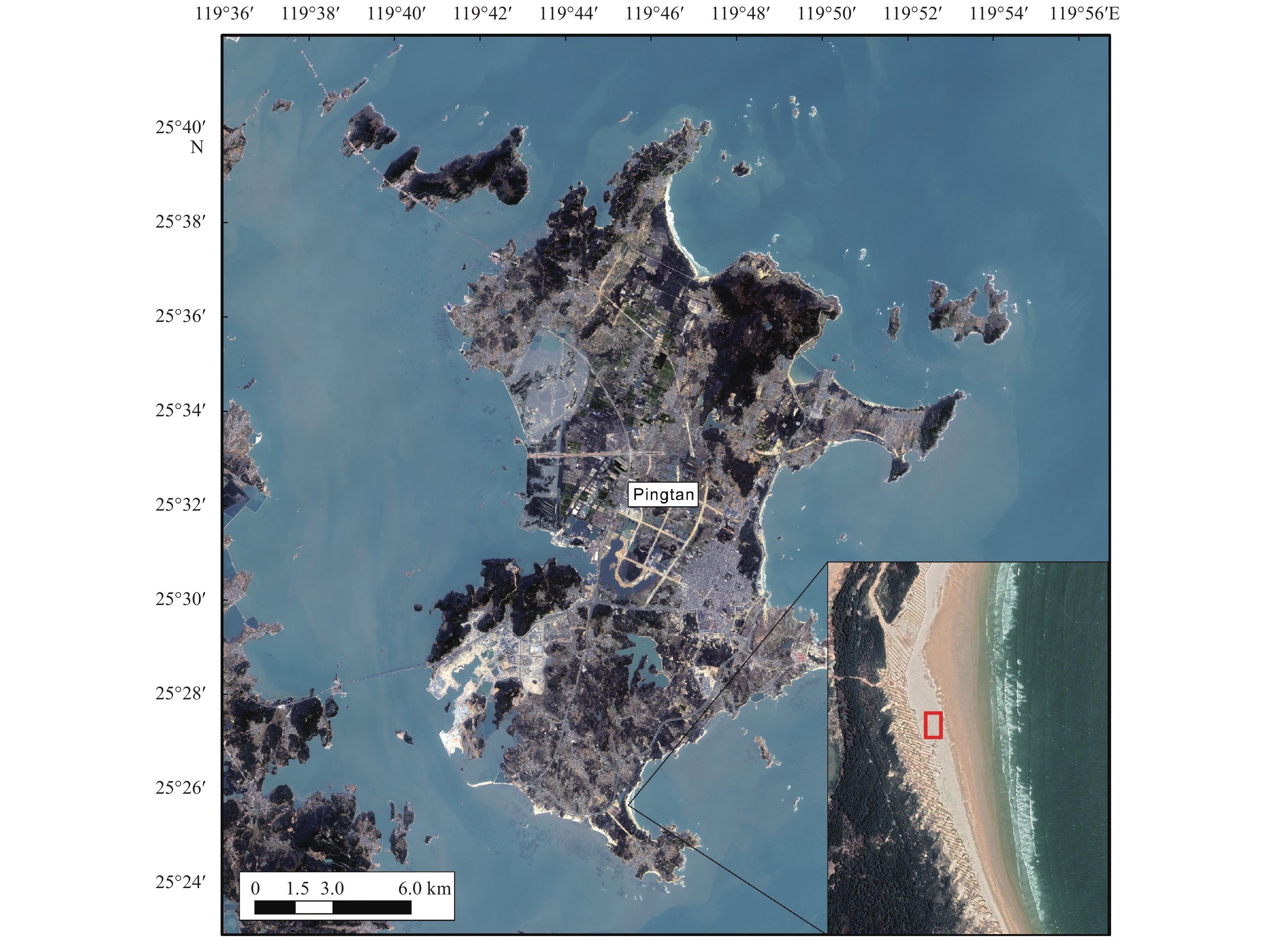
Map of study site (data source: Google Earth).
| Citation: | Qingqian Ning, Bailiang Li, Changmao Zhou, Yanyu He, Jianhui Liu. Effect of fence opening configurations on dune development[J]. Acta Oceanologica Sinica, 2023, 42(7): 185-193. doi: 10.1007/s13131-023-2192-8

|
Wind-blown sediment transport is a ubiquitous process on Earth and many other planetary surfaces such as Mars and Venus. In addition to land forming, it can also bring many aeolian hazards, such as soil nutrients removal (Wen and Zhen, 2020), infrastructure damage (Hassan and Guirguis, 2013; Mehdipour and Baniamerian, 2019), and human respiratory system impairment (Li and Sherman, 2015; Middleton, 2017), which will be even worse in the highly populated coastal areas, where one-third of the human population lives (Gittman et al., 2016; Currin, 2019).
Fences have been widely used to mitigate aeolian erosion and to initiate deposition due to its low cost and easy deployment (Itzkin et al., 2020). As a soft engineering approach, fence construction can be easily integrated into the coastal ecosystem, which is a nature-based strategy for foredune re-establishment (Miller et al., 2001). Fences, together with newly built dune ridges, can substantially reduce the onshore sand drift, which, therefore, minimizes the risks to bury roads, buildings, and ecological features like coastal forests and wetland (Borsje et al., 2011; Hotta and Horikawa, 1991; Sherman and Nordstrom, 1994).
It is widely believed that sand fences can control the sand deposition and dune development (Nordstrom and Jackson, 2018; Jackson and Nordstrom, 2018; Itzkin et al., 2020), and fences with different configurations such as porosity, opening size, and height can have very different trapping effects (Li and Sherman, 2015). Fence porosity of around 40%–50% is commonly considered optimal in terms of sand trapping (Hotta and Horikawa, 1991; Bofah and Al-Hinai, 1986; Mendelssohn et al., 1991). However, the effect of opening size on trapping effect is rather limited and only one wind tunnel work on slat fences shows that fences with smaller slat gaps appear to have higher trapping efficiency than those with larger gaps (Manohar and Bruun, 1970). According to a recent field study trapping capacity is considered proportional to fence height (Ning et al., 2020).
However, studies on opening geometry and porosity distribution effects on sand trapping is rather limited. We only locate one wind tunnel study, which demonstrates that slat fences with smaller gaps have higher trapping efficiency (Manohar and Bruun, 1970). Most relevant studies are focused more on their wind reduction effect rather than their sand trapping effect. For example, Wang et al. (2018) found punch plate fence (circular holes) has larger wind reduction than wire mesh fence (rectangular holes) in a wind tunnel study. Park and Sang (2001) found that fences with non-uniform porosity distribution have a smaller shelter effect than fence with uniform porosity, however, it was challenged by a later study (Cornelis and Gabriels, 2005) that uniform fences have more significant shelter effect. As wind reduction controls sand deposition, it is therefore expected that these fence configurations also have strong influence on sand trapping.
Therefore, the effect of opening size, geometry, and orientation, and porosity distribution on sand trapping have been clearly understudied. In this paper, we will conduct a series of field experiments to address how fence opening configurations affect dune development.
The field experiment was conducted from Dec. 2017 to Mar. 2018 on a dry, flat beach (25°25′32.48′′N, 119°45′0.01′′E) at the Yuandang Bay, Pingtan, China (Fig. 1), with NNE–NE in prevailing wind direction and active sand transport in winter (He et al., 2022). The nearshore has an annual wave height of 1.1 m and a typical tidal range of 5 m and the sand is well-sorted with median grain size of 0.25–0.45 mm (He et al., 2022).
Eight fences with different configurations were prepared for the field experiment: Large Grid (LG), Rotated Large Grid (RLG), Horizontal Slat (HS), Vertical Slat (VS), Medium Grid (MG), Small Grid (SG), Upper Denser (UD), and Lower Denser (LD) (c.f. Table 1). LG and RLG has the opening size of 70 mm × 70 mm, HS has the gap size of 30 mm × 570 mm, VS has the gap size of 30 mm × 470 mm, MG and SG have the opening size of 50 mm × 50 mm, and 30 mm × 30 mm, respectively. The denser section of UD and LD has the opening size of 20 mm × 60 mm and porosity of 36% while sparser section has 60 mm × 260 mm opening size and 61.7% porosity. LG, MG and SG fences are used to examine the opening size effect. LG vs. RLG and HS vs. VS are used to investigate the orientation effect. UD and LD are used to evaluate the porosity distribution effect.
| Fence type | Large Grid | Rotated Large Grid | Horizontal Slat | Vertical Slat |
| Fence porosity | 48.0% | 48.0% | 48.7% | 51.7% |
| Fence drawing |  |  |  |  |
| Fence type | Medium Grid | Small Grid | Upper Denser | Lower Denser |
| Fence porosity | 50.2% | 51.6% | 49.3% | 49.3% |
| Fence drawing |  |  |  |  |
 DownLoad:
CSV
DownLoad:
CSV
The fences were manufactured with 3 mm thick square plywood boards with dimension of 600 mm × 600 mm. For each type of fence, 18 fence pieces were connected and aligned to form the continuous fence with a total length of 10.8 m. The bottom 100 mm of each fence piece was buried in the sand and the remaining height of each fence piece above the leveled terrain surface was 50 mm. After the burial, the exposed sections have similar porosities ranging from 48% to 51.7% (c.f. Table 1) and the length to height ratio of all eight fences was 21.6, well beyond the criteria of 13, which is recommended by Bofah and Al-Hinai (1986), to avoid the edge effect on the dune formation along the fence centerline.
Four sets of experiments were conducted and for each experiment, one seaward fence and one landward fence were deployed at the study site (c.f. Table 2). As shown in Fig. 2, both fences were deployed side by side, with their orientation approximately perpendicular to the prevailing wind direction (c.f. Fig. 2), and the gap between the closest fence edges were about 5 m.
| Experiment number | Landward fence | Seaward fence | Start date | End date | Topography measuring method | |||
| Fence type | Porosity | Fence type | Porosity | |||||
| 1 | LG | 48.0% | RLG | 48.0% | Dec. 25, 2017 | Jan. 9, 2018 | TLS | |
| 2 | HS | 48.7% | VS | 51.7% | Jan. 11, 2018 | Jan. 15, 2018 | TLS | |
| 3 | MG | 50.2% | SG | 51.6% | Jan. 23, 2018 | Jan. 31, 2018 | Erosion Pins | |
| 4 | UD | 49.3% | LD | 49.3% | Feb. 1, 2018 | Apr. 11, 2018 | TLS | |
| Note: LG: Large Grid; HS: Horizontal Slat; MG: Medium Grid; UD: Upper Denser; RLG: Rotated Large Grid; VS: Vertical Slat; SG: Small Grid; LD: Lower Denser; TLS: Terrain Laser Scanner. | ||||||||
DownLoad:
CSV

Terrain Laser Scanner (TLS) Leica Scanstation P40 was installed on a tripod to obtain the topographic change around the two fences at a vertical resolution of 0.8 mm for Experiments 1, 2 and 4. For the first two experiments, the tripod was located on a dune top around 60 m away from the closest fence, with the center of the scanner view on the extension line of the two fences so that fences could not block the view. For the last experiment, the tripod was located between the two fences, with the view center still on the extension line. Scanning started normally right after the fences were established, and was repeated when there was an obvious topography change.
For the Experiment 3, erosion pins with mark interval of 1.8 cm were deployed to record the dune development due to the technical problems of the TLS. The erosion pins were located at the centerline of each fence at 0.5 m, 1 m, 2 m, 3 m, and 4 m upwind and 0.3 m, 0.6 m, 1 m, 1.5 m, 2 m, 2.5 m, 3 m, 3.5 m, and 4 m downwind from the fence. The topography change was estimated by examining the variations of the exposed marks.
To obtain wind velocity profile and wind direction, a meteorological tower was installed with one cup anemometer (Yigu Sci, YGC-FS) at 0.880 m and a wind vane (Yigu Sci, YGC-FX) at 2.183 m above ground (c.f. Fig. 2). Wind was measured continuously and then block-averaged at an interval of 5 min.
To determine the threshold velocity, a saltation sensor (Sensit H14-LIN) was deployed spanwisely, about 0.2 m from the tower. A vertical stack of sand traps were deployed near the Sensit to collect sand transport within 30 cm above the surface. There were totally 10 trap runs conducted from Feb. 1 to 5, 2018. The trap run information including deployment time and duration, and total sand weight is summarized in Table 3.
| Trap run number | Date and starting time | Run duration T/s | Average wind speed U/(m·s–1) | Total sand weight M/g | Average sand transport rate Q/(g·m–1·s–1) |
| 1 | Feb. 1, 19:02:30 | 360 | 6.38 | 43.06 | 1.20 |
| 2 | Feb. 1, 19:17:05 | 420 | 13.13 | 74.93 | 1.78 |
| 3 | Feb. 1, 19:35:05 | 360 | 2.82 | 3.42 | 0.09 |
| 4 | Feb. 1, 19:49:30 | 540 | 9.95 | 75.79 | 1.40 |
| 5 | Feb. 2, 10:25:50 | 360 | 4.01 | 33.61 | 0.93 |
| 6 | Feb. 4, 10:54:30 | 240 | 10.38 | 98.62 | 4.11 |
| 7 | Feb. 4, 11:11:30 | 300 | 21.80 | 212.48 | 7.08 |
| 8 | Feb. 4, 11:31:10 | 240 | 16.96 | 93.36 | 3.89 |
| 9 | Feb. 5, 15:59:30 | 570 | 10.73 | 92.01 | 1.61 |
| 10 | Feb. 5, 16:20:00 | 600 | 9.41 | 36.55 | 0.61 |
DownLoad:
CSV
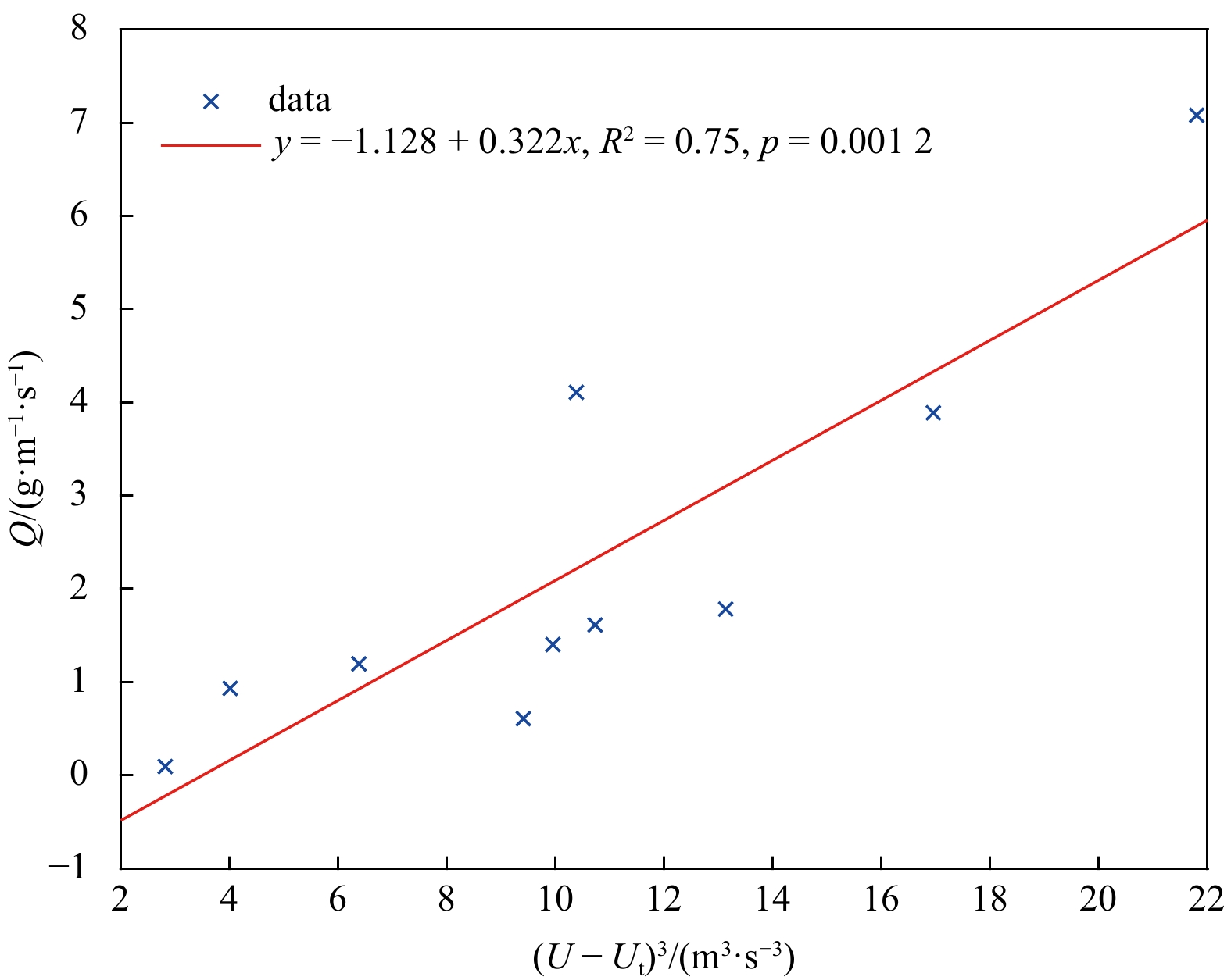
With the trap data, the average sediment transport rate Q for each trap run can be calculated using
| $$ Q=\frac{M}{WT} \ , $$ | (1) |
where M is the total sand weight (g), T is the trap run duration (s), and W is the trap width of 0.1 m. After calculating the average wind speed U for each block (c.f. Table 3), a linear relationship between (U – Ut)3 and Q can be derived as shown in Fig. 3. Note here Ut is the threshold velocity of 3.4 m/s, which is defined as the wind speed where the Sensit signals transit from zero to non-zero. With this relationship, the sediment transport rate for each 5 min block can be estimated. Therefore, the accumulated incoming sand flux Ft (in g/m) at time t can be derived using

| $$ {F}_{{t}}={\sum }_{i=1}^{t/{T}_{\mathrm{b}}}{Q}_{i}{T}_{\mathrm{b}}={T}_{\mathrm{b}}{\sum }_{i=1}^{t/{T}_{\mathrm{b}}}{Q}_{i} \ , $$ | (2) |
where
TLS Data were imported into Leica Geosystems 9.1 (version 9.1.6 64-bit build 5603) and xyz point clouds data were exported after registration, plane unification, and unnecessary region removal. For the convenience of topography change evaluation, the point clouds were shifted and rotated to make new x axis falling on the fence line with positive pointing landward, new y axis pointing downwind, and new z axis pointing upward. Note y = 0 is located at the fence line, z = 0 is located at the foot level of the fences, i.e., 0.5 m lower than the fence tops. The centerline topographic profiles on the y-z plane for each fence were derived after interpolating z values with y interval of 0.01 m. As the initial plane is not perfectly flat, to accurately estimate the sand deposit, each profile was subtracted by its initial profile derived from the first scan of each experiment. Similarly, the topographic profiles measured by erosion pins were also subtracted by the initial profiles for Experiment 3. After the subtraction, topographic profile area At (m2) at time t can be estimated, which can be used to calculate the accumulated deposition volumes (m3) for a unit width of 1 m from start of each experiment Vt by
| $$ {V}_{\mathrm{t}}={A}_{{t}}\times 1\;{\rm{m}}\ . $$ | (3) |
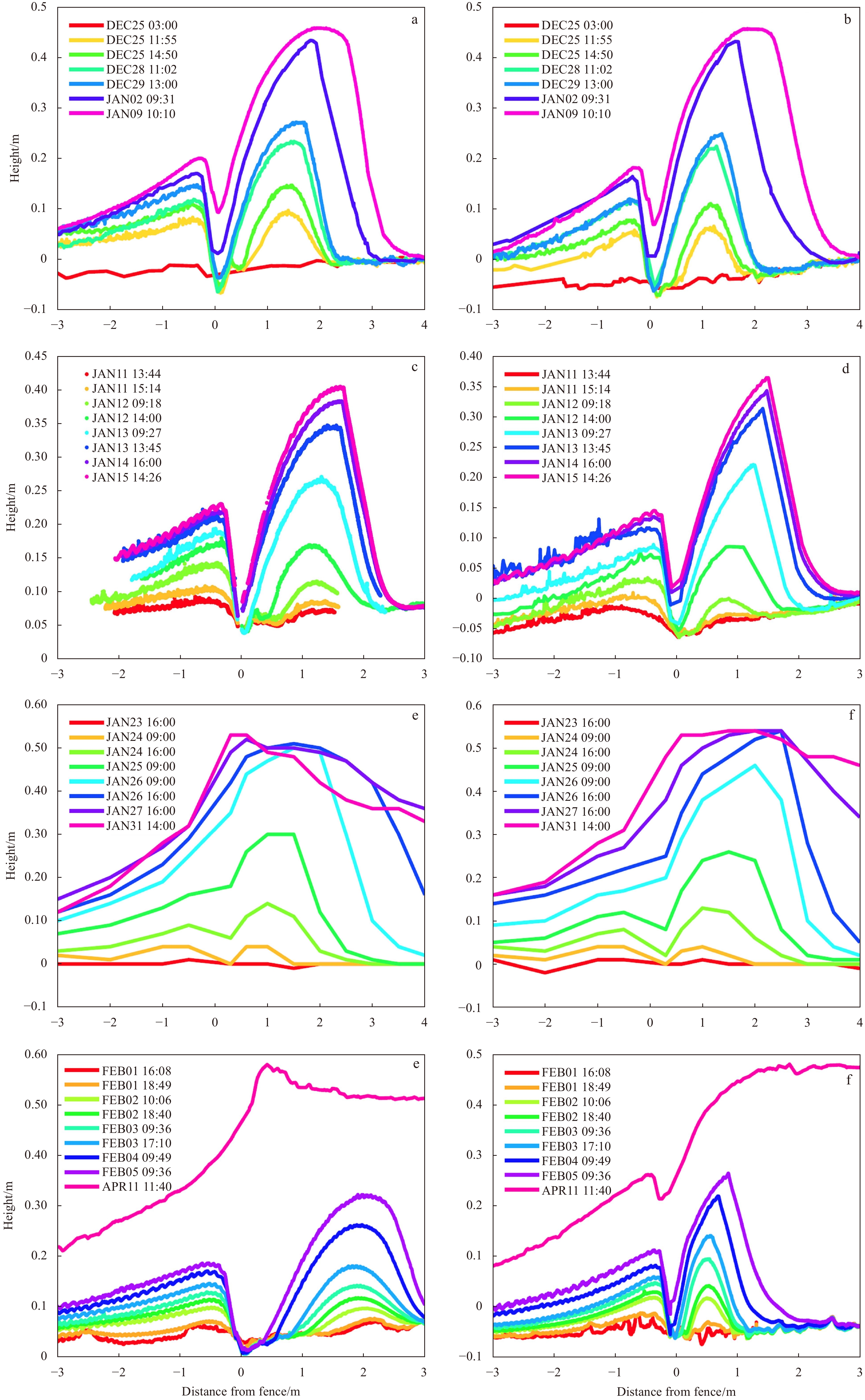
Ning et al. (2020) observed two stages of dune development around fences. In Stage I, the dune grows vertically to reach the maximum height, and in Stage II the dune grows horizontally to expand the dune crest. For Experiments 1 and 2, we only observe the dune development in Stage I (c.f. Figs 4a–d) due to limited sand supply. However, for Experiments 3 and 4, dunes had entered Stage II and even stopped growing after their last measurements (c.f. Figs 4e–h), indicating they reached an equilibrium status.

As shown in Fig. 4, for all cases, there emerged two dunes on windward and leeward sides of each fence, respectively, after sand started to move. All windward dunes were much smaller than the leeward dunes. For each fence, there is a distinct trough between these two dunes except for the cases of MG and SG, when erosion pins were used, maybe because of the lack of erosion pin deployment at the fences. The trough is deeper for HS and UD than their counterparts VS and LD, respectively. For all fences, the profile patterns of windward dunes were very similar to each other and their occurrence locations are quite close while for the leeward dunes, their profiles varied both in location and geometry. These two dunes start to merge during Stage II and finally only a small trough was observed at LD fence while no observable trough for UD fence.
As shown in Fig. 4, although the general patterns of the dune development is similar between fences, the specific dune crest locations can be very different. To explore this, we have plotted the peak locations with distance to fence as x and height as y in Stage I (Fig. 5). As shown in the Fig. 5a, most of windward dune peaks are located between −1 m and 0 m, with distance almost as a constant for most of fences except HS, MG and SG, demonstrating almost the vertical growth in Stage I. The sudden increase of peak distance may be due to the scanning error induced abrupt local topography change as shown in Fig. 4d. For MG and SG fences, as mentioned before, their peaks may not be correctly identified due to the low spatial resolution of erosion pins. The UD fence also has the longest distances compared to other fences.

As shown in Fig. 5b, after some initial adjustments, the most leeward dunes have slight tendency to move downwind with increase of dune height except for UD fence which has the opposite trend. Moreover, peak distance has more variability than windward cases. For example, UD fence has the longest distances and LD fence has the shortest distance. SG fence has longer distance than LD but smaller than other fences. For most heights, there are insignificant differences in distance among LG, RLG, HS, VS, and MG.
With the development of the dune, the windward dune and leeward dune are prone to merge into one large dune during the Stage II. Figure 6 demonstrates the last profiles for MG, SG, UD and LD fences. MG and LD fences have flatter crest with more downwind peak locations than SG and UD. The peak height has the order of UD > MG > SG > LD, same as the order of the cross-sectional areas, indicating UD and MG has larger trapping capacity.

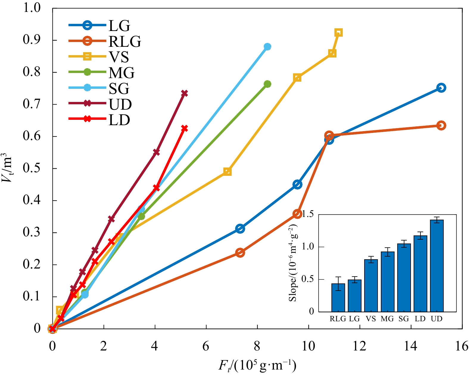
The accumulated deposition volumes Vt in Stage I is plotted against accumulated incoming sand flux Ft at time t (c.f. Fig. 7). Statistical analysis shows that there are linear relationships between them for all fences at 95% confidence level. The slope of these curves represents the ratio of deposited sand to incoming sand, therefore, it can be used to as a proxy to represent the trapping efficiency. As shown in the subplot of Fig. 7, the trapping efficiency has the order of UD > LD > SG > MG > VS > LG and RLG, showing fences with small, non-uniform porosity have higher trapping efficiency than fences with large, uniform porosity.

Here we propose a framework to demonstrate the interactions between wind, fence, sand, and dunes based on previous relevant aerodynamic works (Plate, 1971; Judd et al., 1996; Dong et al., 2006). As shown in Fig. 8, at the beginning of Stage I, the incoming sand-laden flow slows down its speed once it approaches the fence, where sand starts to deposit. However, when the flow passes through the fence openings, it is split and accelerated into numerous jets and thus almost no sand deposition at the fence. However, as the air behind the solid area of the fences is still, the spatially averaged wind speed in the near lee is low, leading to sand deposition where the jets are merged downwind. There is a flow separation at the fence top, generating a strong shear flow downwind, and this flow reattaches ground and stops sand deposition in the farther lee. The two deposition zones result in the formation and growth of the two dunes with a trough area in between. As the vertical growth of windward dune, the wind shadow area becomes larger and larger, thus weakening the jet flows, especially near the ground. This leads to more deposition in the trough area, and the two dunes start to merge. At the end of Stage I, the vertical growth of leeward dune stops due to the strong shear flow at the fence top level while the windward dune continues to grow vertically, which keeps enlarging the wind shadow area, resulting the continuous sand filling in the trough. Finally, the two dunes completely merge at the fence and form an equilibrium dune profile at the end of Stage II, when fence is almost buried with wind shear between impact threshold and fluid threshold across the whole profile and no further deposition or erosion occurs. It is obvious that the introduction of fence into the aeolian system makes the original wind-sand-dune system a three-way interaction into a wind-fence-sand-dune four-way interaction. This makes the fenced dune’s equilibrium profile looks substantially different from unfenced mature dune profile (c.f. last two dunes in Fig. 8). Moreover, unlike the fenced dune that has fixed location, the unfenced dune is still migrating due to continuous erosion on the stoss slope and deposition on the lee slope (Kocurek et al., 1992). However, as the wind field was not measured during the experiments, this framework is hypothetical and should be further examined.

The porosity of all the eight fences are designed to be around 50%. As porosity is considered as the primary control of wind field (Li and Sherman, 2015), similar air flows are expected to be formed. Therefore, it is not surprising to see all fences have similar two-dune-one-trough patterns. Although the dune development process shows little difference for some fences, we have also found that some fences have significant different dune profiles, especially in the near lee, which should be attributed to different configurations because porosity distribution, opening size, and opening geometry mostly affect the flows near fences (Jensen, 1954; Li and Sherman, 2015).
The dune profiles of LG and RLG fences are very similar to each other. This indicates the impact of opening orientation in this case (45° rotation) on the wind field was not significant. However, the HS fence and VS fence (90° rotation) have detectable impact on the profiles very close to the fences while the profiles in other places are very close. This may be because the horizontal slats create a continuous gap parallel to the surface, which allows the jets flows always greater than the threshold. However, for vertical slat, as flows were split into vertical jets, near surface flows are generally weaker, allowing more sand deposition at the fence. Compared to other fences, UD fence has the largest opening size near surface. This makes the surface wind reduction is generally smaller which leads to the largest trough area between the two peaks.
The dune peak heights from this study (0.8 to 1.2 times of fence height) is compatible with the results of other sand fence studies (Hotta and Horikawa, 1991; Tabler, 1980; Iversen, 1981; Ning et al., 2020). This is mainly because there is a strong shear flow at the level of fence height (Ning et al., 2020). However, the distance of the leeward peak to fence is apparently controlled by the configurations of fences. Fences with smaller openings, such as SG and LD fences, appears more effective in trapping sand closer to fence during Stage I, which is consistent with previous studies (Hotta and Horikawa, 1991) . This is mainly due to their stronger reduction effect on wind speed (Dong et al., 2011).
Fences with non-uniform porosities tend to have the largest trapping efficiency and fences with larger grids have the smaller efficiency during Stage I. This is consistent with a previous study that slat fences with smaller gaps have higher efficiency (Manohar and Bruun, 1970). This may be also because fences with smaller porosities are more efficient in wind reduction and thus sand deposition. Considering sand transport is proportional to wind speed cubed (Bagnold, 1941), with the similar porosity, fences with more smaller grids can have higher trapping efficiency. With similar reasons, the UD fences can trap most sand than other fences because it had the smallest opening after sand buried the lower section of these fences. However, after the whole fence is buried, the ultimate topographic profile can be only determined after understanding how newly formed dunes interact with sand-laden flows.
The erosion pins utilized in the third experiment leads to low resolution of the profile measurements in the third experiment, which makes it harder to compare with results from other experiments. Another limitation of this study was the inadequate scan area for dunes around HS fence, making it impossible to derive its trapping efficiency. Although the final stage of the UD and LD fences were recorded, the duration from the end of Stage I to the fully developed status was not captured by TLS.
The findings from this study indicate that UD fence is probably an optimal design for sand trapping efficiency and sand trapping capacity. Moreover, the peak of its fully merged dune is at the same location of the fence, which would be convenient for researchers and engineers to deploy the fence at the desired location of the dune.
In this study, field experiment was conducted to investigate the effect of fence configuration on the dune development. Our experiments show that fence configurations not only affect where the dunes would emerge at the beginning but also where and how the dune would appear in the end. Four major conclusions can be drawn:
(1) A similar two-dune-one-trough pattern was found for all fences during the first stage of dune development.
(2) Opening size, orientation, and geometry, and porosity distribution control the locations of the leeward dune peak.
(3) Fences with smaller openings and non-uniform porosity tend to have higher trapping efficiency than those with large openings and uniform porosity.
(4) Upper denser fences have the highest trapping capacity among the fences we studied.
|
Bagnold R A. 1941. The Physics of Blown Sand and Desert Dunes. London: Methuen
|
|
Bofah K K, Al-Hinai K G. 1986. Field tests of porous fences in the regime of sand-laden wind. Journal of Wind Engineering and Industrial Aerodynamics, 23: 309–319. doi: 10.1016/0167-6105(86)90051-6
|
|
Borsje B W, Van Wesenbeeck B K, Dekker F, et al. 2011. How ecological engineering can serve in coastal protection. Ecological Engineering, 37(2): 113–122. doi: 10.1016/j.ecoleng.2010.11.027
|
|
Cornelis W M, Gabriels D. 2005. Optimal windbreak design for wind-erosion control. Journal of Arid Environments, 61(2): 315–332. doi: 10.1016/j.jaridenv.2004.10.005
|
|
Currin C A. 2019. Living shorelines for coastal resilience. In: Perillo G M E, Wolanski E, Cahoon D R, eds. Coastal Wetlands. Amsterdam: Elsevier, 1023–1053
|
|
Dong Zhibao, Luo Wanyin, Qian Guangqiang, et al. 2011. Evaluating the optimal porosity of fences for reducing wind erosion. Sciences in Cold and Arid Regions, 3(1): 1–12
|
|
Dong Zhibao, Qian Guangqiang, Luo Wanyin, et al. 2006. Threshold velocity for wind erosion: the effects of porous fences. Environmental geology, 51(3): 471–475. doi: 10.1007/s00254-006-0343-9
|
|
Gittman R K, Scyphers S B, Smith C S, et al. 2016. Ecological consequences of shoreline hardening: a meta-analysis. BioScience, 66(9): 763–773. doi: 10.1093/biosci/biw091
|
|
Hassan M A, Guirguis N M. 2013. Effect of upstream fencing on shelter zone behind solid models simulating sand formations and dunes. HBRC Journal, 9(1): 93–101. doi: 10.1016/j.hbrcj.2013.02.004
|
|
He Yanyu, Liu Jianhui, Cai Feng, et al. 2022. Aeolian sand transport influenced by tide and beachface morphology. Geomorphology, 396: 107987. doi: 10.1016/j.geomorph.2021.107987
|
|
Hotta S, Horikawa K. 1991. Function of sand fence placed in front of embankment. In: 22nd International Conference on Coastal Engineering. Delft: American Society of Civil Engineers, 2754–2767
|
|
Itzkin M, Moore L J, Ruggiero P, et al. 2020. The effect of sand fencing on the morphology of natural dune systems. Geomorphology, 352: 106995. doi: 10.1016/j.geomorph.2019.106995
|
|
Iversen J D. 1981. Comparison of wind-tunnel model and full-scale snow fence drifts. Journal of Wind Engineering and Industrial Aerodynamics, 8(3): 231–249. doi: 10.1016/0167-6105(81)90023-4
|
|
Jackson N L, Nordstrom K F. 2018. Aeolian sediment transport on a recovering storm-eroded foredune with sand fences. Earth Surface Processes and Landforms, 43(6): 1310–1320. doi: 10.1002/esp.4315
|
|
Jensen M. 1954. Shelter Effect Investigations into the Aerodynamics of Shelter and its Effects on Climate and Crops. Copenhagen: Danish Technical Press
|
|
Judd M J, Raupach M R, Finnigan J J. 1996. A wind tunnel study of turbulent flow around single and multiple windbreaks, part I: velocity fields. Boundary-Layer Meteorology, 80(1–2), 127–165
|
|
Kocurek G, Townsley M, Yeh E, et al. 1992. Dune and dune-field development on Padre Island, Texas, with implications for interdune deposition and water-table-controlled accumulation. Journal of Sedimentary Research, 62(4): 622–635
|
|
Li Bailiang, Sherman D J. 2015. Aerodynamics and morphodynamics of sand fences: A review. Aeolian Research, 17: 33–48. doi: 10.1016/j.aeolia.2014.11.005
|
|
Manohar M, Bruun P. 1970. Mechanics of dune growth by sand fences. Dock and Harbour Authority, 51: 243–252
|
|
Mehdipour R, Baniamerian Z. 2019. A new approach in reducing sand deposition on railway tracks to improve transportation. Aeolian Research, 41: 100537. doi: 10.1016/j.aeolia.2019.07.003
|
|
Mendelssohn I A, Hester M W, Monteferrante F J, et al. 1991. Experimental dune building and vegetative stabilization in a sand-deficient barrier island setting on the Louisiana Coast, USA. Journal of Coastal Research, 7(1): 137–149
|
|
Middleton N J. 2017. Desert dust hazards: A global review. Aeolian Research, 24: 53–63. doi: 10.1016/j.aeolia.2016.12.001
|
|
Miller D L, Thetford M, Yager L. 2001. Evaluation of sand fence and vegetation for dune building following overwash by Hurricane Opal on Santa Rosa Island, Florida. Journal of Coastal Research, 17(4): 936–948
|
|
Ning Qingqian, Li Bailiang, Ellis J T. 2020. Fence height control on sand trapping. Aeolian Research, 46: 100617. doi: 10.1016/j.aeolia.2020.100617
|
|
Nordstrom K F, Jackson N L. 2018. Offshore aeolian sediment transport across a human-modified foredune. Earth Surface Processes and Landforms, 43(1): 195–201. doi: 10.1002/esp.4217
|
|
Park C W, Song J L. 2001. The effects of a bottom gap and non-uniform porosity in a wind fence on the surface pressure of a triangular prism located behind the fence. Journal of Wind Engineering and Industrial Aerodynamics, 89(13): 1137–1154. doi: 10.1016/S0167-6105(01)00105-2
|
|
Plate E J. 1971. The aerodynamics of shelter belts. Agricultural Meteorology, 8: 203–222. doi: 10.1016/0002-1571(71)90109-9
|
|
Sherman D J, Nordstrom K F. 1994. Hazards of wind-blown sand and coastal sand drifts: a review. Journal of Coastal Research, (12): 263–275
|
|
Tabler R D. 1980. Geometry and density of drifts formed by snow fences. Journal of Glaciology, 26(94): 405–419. doi: 10.3189/S0022143000010935
|
|
Wang Tao, Qu Jianjun, Ling Yuquan, et al. 2018. Shelter effect efficacy of sand fences: A comparison of systems in a wind tunnel. Aeolian Research, 30: 32–40. doi: 10.1016/j.aeolia.2017.11.004
|
|
Wen Xin, Zhen Lin. 2020. Soil erosion control practices in the Chinese Loess Plateau: A systematic review. Environmental Development, 34: 100493. doi: 10.1016/j.envdev.2019.100493
|

Figures(8) / Tables(3)

Supported by:
Beijing Renhe Information Technology Co. Ltd


| Fence type | Large Grid | Rotated Large Grid | Horizontal Slat | Vertical Slat |
| Fence porosity | 48.0% | 48.0% | 48.7% | 51.7% |
| Fence drawing | | | | |
| Fence type | Medium Grid | Small Grid | Upper Denser | Lower Denser |
| Fence porosity | 50.2% | 51.6% | 49.3% | 49.3% |
| Fence drawing | | | | |
DownLoad:
CSV
| Experiment number | Landward fence | Seaward fence | Start date | End date | Topography measuring method | |||
| Fence type | Porosity | Fence type | Porosity | |||||
| 1 | LG | 48.0% | RLG | 48.0% | Dec. 25, 2017 | Jan. 9, 2018 | TLS | |
| 2 | HS | 48.7% | VS | 51.7% | Jan. 11, 2018 | Jan. 15, 2018 | TLS | |
| 3 | MG | 50.2% | SG | 51.6% | Jan. 23, 2018 | Jan. 31, 2018 | Erosion Pins | |
| 4 | UD | 49.3% | LD | 49.3% | Feb. 1, 2018 | Apr. 11, 2018 | TLS | |
| Note: LG: Large Grid; HS: Horizontal Slat; MG: Medium Grid; UD: Upper Denser; RLG: Rotated Large Grid; VS: Vertical Slat; SG: Small Grid; LD: Lower Denser; TLS: Terrain Laser Scanner. | ||||||||
DownLoad:
CSV
| Trap run number | Date and starting time | Run duration T/s | Average wind speed U/(m·s–1) | Total sand weight M/g | Average sand transport rate Q/(g·m–1·s–1) |
| 1 | Feb. 1, 19:02:30 | 360 | 6.38 | 43.06 | 1.20 |
| 2 | Feb. 1, 19:17:05 | 420 | 13.13 | 74.93 | 1.78 |
| 3 | Feb. 1, 19:35:05 | 360 | 2.82 | 3.42 | 0.09 |
| 4 | Feb. 1, 19:49:30 | 540 | 9.95 | 75.79 | 1.40 |
| 5 | Feb. 2, 10:25:50 | 360 | 4.01 | 33.61 | 0.93 |
| 6 | Feb. 4, 10:54:30 | 240 | 10.38 | 98.62 | 4.11 |
| 7 | Feb. 4, 11:11:30 | 300 | 21.80 | 212.48 | 7.08 |
| 8 | Feb. 4, 11:31:10 | 240 | 16.96 | 93.36 | 3.89 |
| 9 | Feb. 5, 15:59:30 | 570 | 10.73 | 92.01 | 1.61 |
| 10 | Feb. 5, 16:20:00 | 600 | 9.41 | 36.55 | 0.61 |
DownLoad:
CSV
| Fence type | Large Grid | Rotated Large Grid | Horizontal Slat | Vertical Slat |
| Fence porosity | 48.0% | 48.0% | 48.7% | 51.7% |
| Fence drawing | | | | |
| Fence type | Medium Grid | Small Grid | Upper Denser | Lower Denser |
| Fence porosity | 50.2% | 51.6% | 49.3% | 49.3% |
| Fence drawing | | | | |
| Experiment number | Landward fence | Seaward fence | Start date | End date | Topography measuring method | |||
| Fence type | Porosity | Fence type | Porosity | |||||
| 1 | LG | 48.0% | RLG | 48.0% | Dec. 25, 2017 | Jan. 9, 2018 | TLS | |
| 2 | HS | 48.7% | VS | 51.7% | Jan. 11, 2018 | Jan. 15, 2018 | TLS | |
| 3 | MG | 50.2% | SG | 51.6% | Jan. 23, 2018 | Jan. 31, 2018 | Erosion Pins | |
| 4 | UD | 49.3% | LD | 49.3% | Feb. 1, 2018 | Apr. 11, 2018 | TLS | |
| Note: LG: Large Grid; HS: Horizontal Slat; MG: Medium Grid; UD: Upper Denser; RLG: Rotated Large Grid; VS: Vertical Slat; SG: Small Grid; LD: Lower Denser; TLS: Terrain Laser Scanner. | ||||||||
| Trap run number | Date and starting time | Run duration T/s | Average wind speed U/(m·s–1) | Total sand weight M/g | Average sand transport rate Q/(g·m–1·s–1) |
| 1 | Feb. 1, 19:02:30 | 360 | 6.38 | 43.06 | 1.20 |
| 2 | Feb. 1, 19:17:05 | 420 | 13.13 | 74.93 | 1.78 |
| 3 | Feb. 1, 19:35:05 | 360 | 2.82 | 3.42 | 0.09 |
| 4 | Feb. 1, 19:49:30 | 540 | 9.95 | 75.79 | 1.40 |
| 5 | Feb. 2, 10:25:50 | 360 | 4.01 | 33.61 | 0.93 |
| 6 | Feb. 4, 10:54:30 | 240 | 10.38 | 98.62 | 4.11 |
| 7 | Feb. 4, 11:11:30 | 300 | 21.80 | 212.48 | 7.08 |
| 8 | Feb. 4, 11:31:10 | 240 | 16.96 | 93.36 | 3.89 |
| 9 | Feb. 5, 15:59:30 | 570 | 10.73 | 92.01 | 1.61 |
| 10 | Feb. 5, 16:20:00 | 600 | 9.41 | 36.55 | 0.61 |
 DownLoad:


 DownLoad: