Figure
1.
Diagram of sources and sinks of Ra in coastal waters. SFGD: submarine fresh groundwater discharge; SPM: suspended particulate matter.
| Citation: | Linwei Li, Jinzhou Du, Xilong Wang, Yanling Lao. Distinguishing the main components of submarine groundwater and estimating the corresponding fluxes based on radium tracing method—taking the Maowei Sea for example[J]. Acta Oceanologica Sinica, 2023, 42(8): 1-23. doi: 10.1007/s13131-023-2211-9

|
The coastal zones are relatively densely populated and economically developed regions in the world where land-ocean interactions occur actively (Canuel et al., 2012). The high intensity human activities cause great pressure to the coastal ecological environment and affect the sustainable development of coastal economy (Pereira-Filho et al., 2001; Ip et al., 2007). Submarine groundwater discharge (SGD) is defined as all the flows from the sea floor to coastal waters in the continental margin, regardless of the composition and driving force (Burnett et al., 2003). SGD can be divided into two types and three main components. The first type is fresh groundwater from the inland (submarine fresh groundwater discharge, SFGD). The second type refers to the water that seeps into the aquifer and then flows back to the sea (recirculated saline groundwater discharge, RSGD) of which the driving is mainly waves (including tide and wind waves) and water density difference. According to different places of occurrence, RSGD can be divided into tidal flat RSGD, which refers to fresh-seawater circulation in intertidal coastal aquifers, and subtidal RSGD, which refers to the water circulation between bottom sediments and overlying water (Huang, 2015; Ma, 2016). As one of the important processes of land-ocean interactions in the coastal zone (LOICZ), SGD has been proved to be another important route for terrigenous materials to enter the sea in addition to surface runoff and atmospheric sedimentation (Moore, 2010a; Charette et al., 2012; Taniguchi et al., 2002). The submarine groundwater has different geochemical characteristics compared with the surface water. Due to the influence of human activities, terrigenous groundwater (Here, mainly refers to SFGD) contains high concentration of nutrients (Burnett et al., 2003; Boehm et al., 2004), carbon (Maher et al., 2013; Liu et al., 2014), methane (Lecher et al., 2016) and heavy metals (Knee and Paytan, 2011). The discharge of these substances into the sea may change of geochemical components of offshore water bodies, which will have adverse effects on the coastal ecological environment (Wang et al., 2014; Liu et al., 2017). After the nearshore seawater penetrating into the coastal aquifer, the salinity of the porewater will be changed, which will lead to the change of reaction rates of some types of chemical reaction in the mixing zone, for example, the ion exchange reaction between solid and liquid phases of the aquifer. Also, carbon, nutrients and other substances will be precipitated. Therefore, RSGD also carries considerable dissolved substances (Gibbes et al., 2008; Anschutz et al., 2009; Santos et al., 2012), but in general, the chemical composition of RSGD is different from that of SFGD and seawater.
The geochemical tracing method can provide the average SGD flux of the study area with less works (Burnett et al., 2001), which is one of the most widely adopted and effective methods for quantitative estimation of SGD fluxes (Wang et al., 2015). Among the tracer, natural radium (Ra) isotopes are one of the widely adopted. In recent years, many studies have reported the SGD fluxes of different types of coasts based on Ra tracing method (Moore et al., 2011; Garcia-Orellana et al., 2014; Wang and Du, 2016; Liu et al., 2017, 2018; Luo et al., 2018).
However, most of the existing studies are based on the basic principle of Ra mass conservation in the study area, and SGD flux is obtained indirectly by evaluating the values of various sources and sinks of Ra in the water. Those methods assume the study area as a “Black Box” and does not care about the spatial distribution of Ra within the “Box” (hence the name “Box model”). Box model is very suitable for semi-enclosed and closed areas such as estuaries, lakes, bays and lagoons with small spatial scale (Su, 2013). However, in bays with larger spatial scales, the Ra activity concentration gradient can be obviously observed in the water bodies, that is, the transport process of Ra exists. In this case, it is not appropriate to treat the study area as a “Black Box”.
In addition, the results obtained by the conventional Ra tracing methods are mostly the average flux of SGD for the whole study area, and few studies distinguish the components of SGD (Liu et al., 2021). As mentioned before, due to the different sources, the chemical compositions of different SGD components may also be different. For the purpose of a more accurate evaluation of the SGD on coastal ecological environment, it is necessary to estimate the fluxes of each component separately.
Advection-diffusion equation (ADE) is a basic model to describe the transport process of solute in the continuous medium, which can describe the space-time distribution of solute in the medium. In order to take full advantage of the information contained in the Ra activity concentration gradient in water, the one-dimensional ADE is adopted as the basic mathematical model in theoretical method. This study is developed on the basis of previous studies (Moore and Arnold, 1996; Swarzenski and Izbicki, 2009; Rodellas et al., 2014). In this study, SFGD and tidal flat RSGD are included in the boundary conditions at the land-sea interface, and subtidal RSGD is taken as one of the source terms of Ra in the ADE. The three components of SGD can be distinguished and their respective fluxes can be obtained. For practice, we choose the Maowei Sea along the northern coast of the Beibu Gulf as the study area, and select 224Ra as the tracer. By the method we proposed the fluxes of three main components of SGD in the Maowei Sea could be calculated respectively.
SFGD and tidal flat RSGD can reflect more information about the impact of terrigenous materials on offshore ecological environment, hence researches pay more attention to them. Compared with the SGD flux in a certain period of time in the study area, the long-term variation trend of SGD is more valuable information. Researches have studied the variation trend of SGD at different time scales by combining field data with Darcy’s law (Wilson et al., 2015), or conducting numerical simulation with hydrological models (Lee et al., 2013; Yu, 2021). Long-term continuous observation of the study area is relatively direct and objective, but it may consume more human and material resources. Numerical models can provide SGD fluxes at different time scales with less field works. However, they are more convenient for ideal coastal aquifer models. In order to conduct modeling analysis for a specific study area, it is still necessary to carry out more field investigation and data search, so as to obtain more accurate topographic information and hydrogeological parameters of the research area. Based on Ra tracing method, this study also proposed a relatively simple but reliable method for long-term monitoring of SFGD and tidal flat RSGD fluxes.
To obtain the accurate values of Ra sources and sinks in coastal water (Fig. 1) is the key to estimate the SGD flux using Ra tracing method (Gu, 2015). The main sources of Ra in the coastal waters are: (1) the dissolved Ra of the river input; (2) Ra adsorbed on suspended particulate matter (SPM) will desorb after contact with salt water; (3) Ra fluxes released by bottom sediments to overlying water including Ra carried by subtidal RSGD and Ra molecular diffusion; (4) the dissolved Ra carried by SGD including the terrigenous dissolved Ra carried by SFGD and the dissolved Ra carried by tidal flat RSGD. Generally, there are mainly two Ra sinks: (1) the offshore transport (Lamontagne and Webster, 2019); (2) the decay loss (Garcia-Orellana et al., 2014), of which the effect is particularly significant for the short-lived Ra isotopes (223Ra, 224Ra). However, for long-lived Ra isotopes (such as 226Ra), especially the spatial scale of the study area is relatively small, the effect of decay may be ignored.
Among Ra isotopes, 224Ra is an ideal tracer for small scale study area (Lamontagne and Webster, 2019). In this study, one-dimensional advection-diffusion equation is adopted to describe the 224Ra activity concentration distribution in coastal water. The contribution of surface runoff and SPM to 224Ra was determined referring to experimental data or literature. Based on the 228Th (the parent nuclide of 224Ra) activity per unit mass of bottom sediment and 224Ra activity concentration distribution in surface seawater in the study area, combined with local wind wave and tide data, the 224Ra flux released by bottom sediments to overlying water was determined as well as the subtidal RSGD flux. On this basis, the SFGD flux and tidal flat RSGD flux could be determined by using the conservation of 224Ra flux at the land-sea interface. The calculation methods used in this article are showed in detail below.
In the sea area where the waves (including tide and wind waves) are strong, the periodic pressure changes caused by waves will make the overlying water penetrate the bottom sediments, and the porewater will also produce a certain velocity upward (Fig. 2). This process formed a circulation between overlying water and porewater, and promoted the turbulent mixing in porewater (Rutgers van der Loeff, 1981). In condition of shallow water depth and high permeability of seafloor sediments, the water exchange between sediment and overlying water interface caused by waves cannot be ignored (Rutgers van der Loeff, 1981). In this paper, the definition of SGD by Burnett et al. (2003) is adopted, thus, the above-mentioned form of water exchange is considered as one kind of SGD.

The turbulent diffusion coefficient (D, m2/s) is used to measure the mixing strength of bottom porewater caused by sea waves:
| $$\tag{1a} D={D}_{0}{{\rm{e}}}^{-2kz} , $$ |
| $$\tag{1b} {D}_{0}=\frac{\pi {K}^{2}_{{z}}T{H}^{2}}{2{ \text{λ} }^{2}{{\rm{cosh}}}^{2}\left(kh\right)} , $$ |
where λ (s−1) is 224Ra decay constant; z (m) is the vertical downward depth of the sediment-overlying water interface; h (m) is the water depth; Kz (m/s) is the vertical hydraulic conductivity of bottom sediment; T (s) is the wave period; H (m) is the tidal range; l (m) is the wave length and
In coastal waters, tidal waves can be approximated as shallow water waves, and the wavelengths (lt, m) can be calculated as follows (Knauss, 1996):
| $$ {l}_{{\rm{t}}}={T}_{{\rm{t}}}\sqrt{gh} , $$ | (2) |
where Tt (s) is tidal cycle; g =9.8 m2/s is the gravitational acceleration.
The wavelength of wind wave (lw, m) should be calculated according to the formula below (Knauss, 1996):
| $$ {l}_{{\rm{w}}{\rm{}}}=\frac{g{T}_{{\rm{w}}}^{2}}{2{\text π} }{\rm{tanh}}\left(\frac{2{\text π} }{{l}_{{\rm{w}}}}h\right) , $$ | (3) |
where Tw (s) is the period of wind wave.
Ra in bottom porewater will migrate into overlying water under diffusion and other mechanisms (Sun and Torgersen, 2001). In addition to turbulent diffusion driven by waves, molecular diffusion caused by random motion of microscopic particles is also an important mechanism of Ra migration in porewater. The molecular diffusion coefficient of Ra (Dm, m2/s) in porewater can be expressed as (Boudreau, 1996)
| $$ {D}_{{\rm{m}}}=\frac{{D}_{{\rm{m}}0}}{1-2\;{\rm{ln}}\left(n\right)} , $$ | (4) |
where Dm0 (8.0×10⁻¹⁰ m2/s) is the molecular diffusion coefficient of Ra in seawater, n is the sediment porosity.
Based on previous studies (Hancock et al., 2000; Nozaki, 1990; Sun and Torgersen, 2001), the following equation is adopted to describe the 224Ra distribution in the bottom sediment porewater:
| $$ n{R}_{{\rm{d}}}\frac{\partial C}{\partial t}=-wn\frac{\partial C}{\partial z}+\left({D}_{{\rm{m}}}+{D}_{{\rm{t}}}+{D}_{{\rm{w}}}\right)n\frac{{\partial }^{2}C}{\partial {z}^{2}}-n \text{λ} C{+p}_{{\rm{v}}}{A}_{{\rm{Th}}}{\rho }_{{\rm{s}}} , $$ | (5) |
where C (m−3) is the 224Ra atom quantity concentration in bottom porewater; w (m/s) is the deposition rate of SPM; Dt (m2/s) and Dm (m2/s) are the turbulent diffusion coefficients driven by tides and wind waves respectively, which can be calculated by Eqs (1), (2) and (3). The dimensionless parameter pv represents the proportion of the volume that contributes to the porewater 224Ra concentration to sediment of characteristic scale volume. The calculation process is detailed in Appendix A. Parameter ATh (Bq/g) is the activity of 228Th in the solid component of bottom sediment per unit mass and ρs (g/cm3) is the density of the solid component of bottom sediment which can be calculated by
| $$ {\rho }_{{\rm{s}}}=\rho /\left(1-n\right) . $$ | (6) |
Retardation factor (Rd) describes the adsorption and desorption of 224Ra by sediment solids, and its expression is as follows:
| $$ {R}_{{\rm{d}}}=1+\frac{\rho }{n}{K}_{{\rm{d}}} , $$ | (7) |
where Kd (cm3/g) is the partition coefficient of 224Ra. It is defined as the ratio of 224Ra activity adsorbed on the sediment surface for per unit mass to 224Ra activity per unit volume of water, and its value is generally related to porewater salinity. In this study, Kd is set to be 840/S, and S is the salinity of porewater (Gu, 2015).
On condition that it is deep enough in the bottom sediment, 224Ra activity in porewater is only controlled by the decay of the parent nuclide in the sediment as well as the adsorption and desorption on the sediment surface. In this case, 224Ra activity reaches equilibrium, that is
| $$ \tag{8a} {\left.\frac{\partial C\left(z,t\right)}{\partial z}\right|}_{z\to \infty }=0 . $$ |
At the sediment-overlying water interface, Ra concentration in porewater is considered to be equal to that in bottom seawater (Csw, m−3):
| $$ \tag{8b}C\left(z,t\right){|}_{z=0}={C}_{{\rm{sw}}} . $$ |
The 224Ra flux released by bottom sediments to overlying water (QB, Bq/(m2·d)) can be calculated as
| $$ {Q}_{{\rm{B}}}=n\text{λ} \left[-wC\left(z,t\right){|}_{z=0}+\left({D}_{{\rm{m}}}+{D}_{{\rm{t}}}+{D}_{{\rm{w}}}\right)\frac{\partial C\left(z,t\right)}{\partial z}{|}_{z=0}\right] , $$ | (9) |
of which the 224Ra flux driven by waves (QB_st, Bq/(m2·d)) are
| $$ {Q}_{{\rm{B}}\_{\rm{st}}}=n\text{λ} \left[\left({D}_{{\rm{t}}}+{D}_{{\rm{w}}}\right)\frac{\partial C\left(z,t\right)}{\partial z}{|}_{z=0}\right] . $$ | (10) |
Numerical method is adopted to solve Eq. (5), so the following approximation can be made:
| $$ \frac{\partial C\left(z,t\right)}{\partial z}{|}_{z=0}=\frac{{C}_{1}-{C}_{0}}{\Delta z} , $$ | (11) |
where C0 and C1 are 224Ra activity values at the first and second space nodes respectively, and
The subtidal RSGD flux (Fst, m3/(m·d)) can be approximated as
| $$ {F}_{{\rm{st}}}=\frac{{Q}_{{\rm{B}}\_{\rm{st}}}}{\left({C}_{1}-{C}_{0}\right)} . $$ | (12) |
After 224Ra enters coastal water from land and seafloor, it will be transported offshore under the mechanism of current and turbulent diffusion (Rengarajan et al., 2002; Colbert and Hammond, 2007). For convenience, the following assumptions were made:
(1) The coastal water depth is relatively shallow; thus, Ra can be considered to be vertically mixed evenly.
(2) Only pay attention to the longitudinal component of the near-sea current field, namely the offshore current, and consider the offshore velocity to be constant within the study scale.
(3) The activity concentration gradient of 224Ra is considered to be approximately perpendicular to the shoreline, that is, 224Ra mainly participates in offshore transport, and the transport flux in parallel shoreline direction can be ignored.
(4) During the study period, the 224Ra activity concentration in seawater reached approximately quasi-steady state.
Based on the above assumptions, one-dimensional steady state advection-diffusion equation can be adopted to describe the 224Ra offshore transport process (Lamontagne and Webster, 2019):
| $$ {D}_{{\rm{L}}}h\frac{{\partial }^{2}{A}_{{\rm{C}}}\left(x\right)}{\partial {x}^{2}}-uh\frac{\partial {A}_{{\rm{C}}}\left(x\right)}{\partial x}- \text{λ} h{A}_{{\rm{C}}}\left(x\right)+{Q}_{{\rm{B}}}=0 , $$ | (13) |
where h (m) is the mean water depth; AC (Bq/m3) is the 224Ra activity concentration in coastal water; λ (s−1) is Ra decay constant; DL (m2/s) is the turbulent diffusion coefficient and u (m/s) is the average net current velocity. Under the assumption of dynamic balance of coastal water volume, u is considered to include the contribution of SFGD and surface runoff as well as the change of water volume caused by precipitation and evaporation (Lamontagne and Webster, 2019):
| $$ u={u}_{{\rm{f}}}+{u}_{{\rm{r}}}+{u}_{{\rm{a}}} , $$ | (14) |
where uf is the velocity contributed by SFGD, and ur is the velocity contributed by surface runoff; ua represents the average current velocity caused by the coastal water budget due to precipitation and evaporation during a certain period, which can be calculated by Lamontagne and Webster (2019):
| $$ {u}_{{\rm{a}}}=\frac{{\int }_{0}^{L}\left(P-E\right)x{\rm{d}}x}{hL}=\frac{\left(P-E\right)L}{2h} , $$ | (15) |
where P (mm/d) is the average precipitation over a period of time in the study area; E (mm/d) is the average evaporation over the same period; and L (m) is the space scale of the sea area studied.
The boundary condition is set to be constant concentration at the land-sea interface.
| $$ \tag{16a}{A}_{{\rm{C}}}\left(x\right){|}_{x=0}={A}_{{\rm{C}}\_0} , $$ |
where AC_0 (Bq/m3) is the 224Ra activity concentration at the land-sea interface.
It is concluded that the 224Ra activity concentration gradient is nearly zero in the water body far enough offshore:
| $$ \tag{16b}\frac{\partial {A}_{{\rm{C}}}\left(x\right)}{\partial x}{|}_{x\to \infty }=0 . $$ |
The analytical solution of Eq. (13) under boundary condition Eq. (16) is
| $$ {A}_{{\rm{C}}}\left(x\right)=\frac{{\text{λ} hA}_{{\rm{C}}\_0}-{Q}_{{\rm{B}}}}{\text{λ} h}{\rm{exp}}\left(-\frac{\sqrt{4{D}_{{\rm{L}}}\text{λ} +{u}^{2}}-u}{2{D}_{{\rm{L}}}}x\right)+\frac{{Q}_{{\rm{B}}}}{\text{λ} h} . $$ | (17) |
The following is the process to estimate the fluxes of tidal flat RSGD and SFGD. At high tide, the seawater seeps into the tidal flat aquifer; at low tide, the infiltrated sea water is discharged with terrigenous freshwater. It is generally believed that the amount of seawater seeped in at high tide is equal to the amount released at low tide after subtraction of fresh groundwater. This process promotes the exchange of materials between land and sea, but the net flux of tidal flat circulation is almost negligible (Ma, 2016). Define the circulation volume between aquifer and sea as tidal flat RSGD, then the 224Ra flux from land to sea is (Qland, Bq/(m·d)):
| $$ {Q}_{{\rm{land}}}={F}_{{\rm{f}}}{A}_{{\rm{C}}\_{\rm{f}}}+{F}_{{\rm{riv}}}{A}_{{\rm{C}}\_{\rm{riv}}}+{Q}_{{\rm{SPM}}}+{F}_{{\rm{tf}}}\left({A}_{{\rm{C}}\_{\rm{pw}}}-{A}_{{\rm{C}}\_0}\right) , $$ | (18) |
where Ff (m3/(m·d)), Ftf (m3/(m·d)) and Friv (m3/(m·d)) are single wide fluxes of SFGD, tidal flat RSGD and surface runoff respectively in study area; AC_f (Bq/m3), AC_riv (Bq/m3) and AC_pw (Bq/m3) are 224Ra activity concentration of fresh ground endmember, river endmember and tidal flat porewater respectively; QSPM (Bq/(m·d)) is the 224Ra flux desorbed from the riverine SPM to seawater, which can be expressed as (Luo, 2018)
| $$ {{Q}}_{{\rm{SPM}}}={F}_{{\rm{riv}}}{C}_{{\rm{SPM}}}{A}_{{\rm{C}}\_{\rm{SPM}}}\eta , $$ | (19) |
where CSPM (g/m3) is the mass concentration of riverine SPM; AC_SPM (Bq/g) is the 224Ra activity of SPM per unit mass; η is the 224Ra desorption ratio of SPM.
The 224Ra offshore transport flux at the land-sea interface (Q0, Bq/(m·d)) is
| $$ {Q}_{0}=uh{A}_{{\rm{C}}\_0}-{D}_{{\rm{L}}}h\frac{\partial A_{\rm{C}}\left(x\right)}{\partial x}{|}_{x=0} . $$ | (20) |
Because of the 224Ra conservation on both sides of the boundary, there is
| $$ {Q}_{0}={Q}_{{\rm{land}}} . $$ | (21) |
According to Eqs (17)–(21), the single wide flux of tidal flat RSGD (Ftf, m3/(m·d)) can be expressed as
| $$ \begin{split}{F}_{{\rm{tf}}}=&[\left({ \text{λ}hA}_{{\rm{C}}\_0}-{Q}_{{\rm{B}}}\right)\sqrt{4{D}_{{\rm{L}}} \text{λ} +{u}^{2}}- \text{λ} (2{F}_{{\rm{f}}}{A}_{{\rm{C}}\_{\rm{f}}}+\\ &2{F}_{{\rm{riv}}}{A}_{{\rm{C}}\_{\rm{riv}}}+2{Q}_{{\rm{SPM}}}-{uhA}_{{\rm{C}}\_0})+\\&u{Q}_{{\rm{B}}}] / [2 \text{λ} ({A}_{{\rm{C}}\_{\rm{pw}}}-{A}_{{\rm{C}}\_0})] . \end{split} $$ | (22) |
According to Eq. (14), the single wide flux of SFGD can be calculated by
| $$ {F}_{{\rm{f}}}=\left(u-{u}_{{\rm{a}}}\right)h-{F}_{{\rm{ri}}{\rm{v}}} . $$ | (23) |
In practice, samples of fresh groundwater can be collected from civil fresh water wells while porewater samples can be collected from tidal flats. At the same time, surface seawater samples will be collected from several stations along the direction perpendicular to the shoreline. Later, 224Ra activity of those samples will be measured in the laboratory. The spatial distribution of 224Ra activity concentration in the coastal water is used to fit Eq. (17) and the undetermined parameters (AC_0, u, DL) can be solved inversely. The other required parameters are relatively easy to be measured on site or obtained from literature. Finally, substitute the parameters and 224Ra activity concentrations of endmembers into Eqs (22) and (23) to calculate the single wide fluxes of tidal flat RSGD and SFGD in the study area.
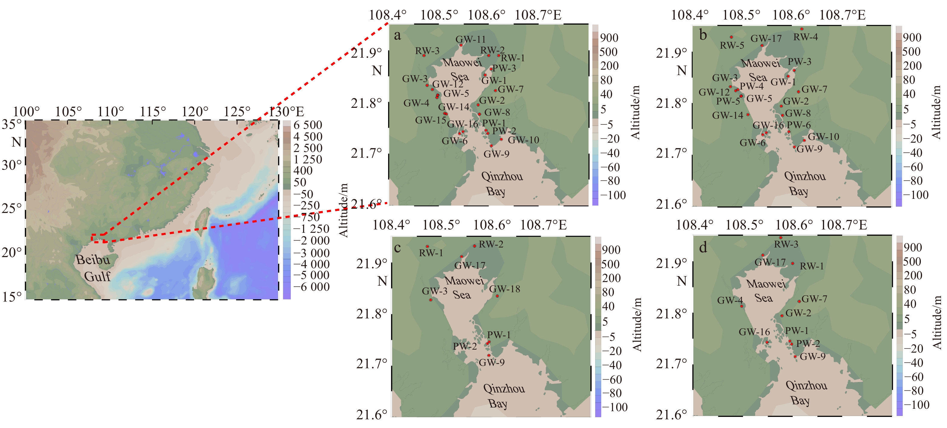
We select the Maowei Sea, located in the north of the Beibu Gulf, as the study area (Fig. 3). This region has a typical subtropical marine monsoon climate, of which the characteristics are: dry season and flood season are distinct, the flood season is hot and rainy, and the winter is short while the summer is long. The average annual temperature in this region is 22–23℃, and the average annual rainfall is 1600–1800 mm. The flood season is mainly from June to August (He, 2015; Li et al., 2001).

The Maowei Sea, which is the inner bay of the Qinzhou Bay, is located at the top of the Beibu Gulf and in the middle of Guangxi coast (21°33'15"–21°54'40"N, 108°28'33"–108°55'53"E). The length of the Maowei Sea from north to south is about 15 km, and the bay mouth is about 2 km wide. The coastline is about 120 km, and the water area is about 135 km2. The average water depth of the Maowei Sea is about 2.5 m, and the water depth is generally not more than 5 m. The Maowei Sea also has a tropical marine monsoon climate with abundant rainfall but great seasonal differences. The average annual temperature of this region is about 22.1℃, while the average annual precipitation is 2140 mm (Tian et al., 2014). The Maowei Sea has an irregular diurnal tide type with an average tidal range of 2.4 m and a maximum range of 5.5 m (Tian et al., 2014). Due to the limitations of topography, the reciprocating flow dominates the tidal current in the Maowei Sea (Zhang, 2010). The Maoling River and the Qinjiang River at the top of the Maowei Sea are the main rivers that flow into the bay. The annual average runoff of the two rivers is 1.6×10¹⁰ m3 and 1.2×10¹⁰ m3, respectively, while the average annual sediment transport is 3.2×10⁵ t and 2.7×10⁵ t, respectively (Xu, 2010). The spatial distribution of surface sediments in the Maowei Sea from the top to the mouth is roughly as follows: sand-silt-clay, clay sand, fine sand (Mo, 1993).
The field works in the Maowei Sea were conducted in June 2016, March 2017, January 2019, and May 2019. Surface water samples, coastal groundwater samples (including fresh ground water and tidal flat porewater), river water samples as well as sediment samples were collected in each sampling period (Fig. 3). Portable multi-parameter was used to measure thermohaline parameters in situ at each station. Later the 224Ra activity of all the samples was measured by Radium Delayed Coincidence Counter (RaDeCC) (Moore and Arnold, 1996).
The measurement results of groundwater and river water samples are shown in Table 1 and the measurement results of surface water in the Maowei Sea are shown in Table 2. Due to the infiltration of seawater into the tidal flat aquifer, the salinity of the tidal flat porewater is significantly higher than that of the fresh groundwater. Also, the 224Ra activity concentration of porewater is higher than that of fresh groundwater overall (the complete experimental data are available in the Appendix B).
| Sample type | Parameter | Sampling date | |||
| June 2016 | March 2017 | January 2019 | May 2019 | ||
| GW AVG | Salinity | 0.2 | 0.2 | 0.2 | 0.2 |
| 224Ra activity concentration/(Bq·m−3) | 35.0 ± 1.6 | 23.6 ± 1.3 | 15.8 ± 1.8 | 8.0 ± 0.8 | |
| PW AVG | Salinity | 15.5 | 19.0 | 23.0 | 26.4 |
| 224Ra activity concentration/(Bq·m−3) | 486.5 ± 16.2 | 299.4 ± 9.0 | 484.4 ± 32.5 | 279.3 ± 14.0 | |
| RIV AVG | Salinity | 0.2 | 0.3 | 2.2 | 1.1 |
| 224Ra activity concentration/(Bq·m−3) | 3.1 ± 0.3 | 3.6 ± 0.3 | 11.2 ± 0.3 | 11.3 ± 1.0 | |
| PW EM | Salinity | 20.1 | 23.4 | 23.0 | 26.4 |
| 224Ra activity concentration/(Bq·m−3) | 486.5 ± 16.2 | 498.0 ± 10.6 | 484.4 ± 32.5 | 279.3 ± 14.0 | |
| Note: AVG means the average value; EM means the end member. | |||||
 DownLoad:
CSV
DownLoad:
CSV
| Parameter | Sampling date | ||||
| June 2016 | March 2017 | January 2019 | May 2019 | ||
| Salinity | Range | 2.5–12.6 | 19.3–25.6 | 13.7–27.9 | 6.6–18.9 |
| AVG | 7.3 | 21.8 | 21.6 | 12.8 | |
| 224Ra/(Bq·m−3) | Range | 7.9–33.0 | 9.9–31.6 | 4.8–13.4 | 5.3–20.2 |
| AVG | 12.8 | 18.3 | 9.1 | 16.1 | |
| Note: AVG means the average value. | |||||
DownLoad:
CSV
In different sampling periods, the salinity of surface seawater in the Maowei Sea showed the same trend that increased from the top to the mouth, indicating that the bay was significantly affected by terrigenous diluted water. The water salinity in the Maowei Sea during the flood season is significantly lower than that during the dry season (Fig. 4). The phenomenon that the water salinity in the bay varies greatly in different seasons, indicating that the terrigenous fresh water flux into the bay may have significant seasonal variation.

The 224Ra activity concentration of surface water in the Maowei Sea had a relatively obvious longitudinal gradient, showing a decreasing trend from land to offshore (Fig. 5). This phenomenon indicates that the land is an important source of 224Ra in the Maowei Sea, and 224Ra mainly participates in the offshore transport under the action of terrigenous fresh water and tidal reversing current.

According to Eq. (1), the turbulent diffusion coefficient in bottom sediment porewater caused by waves is not only related to the properties of waves (wavelength and wave period), but also to the vertical hydraulic conductivity (Kz) of sediments. Once the study area is determined, the wave-related parameters are relatively easy to determine, while the Kz of bottom sediment is relatively difficult to measure in situ. Given this, this section first conducts a sensitivity analysis of Kz to evaluate its influence on the target physical quantities. The parameters obtained during the sampling period in June 2016 were selected as reference for sensitivity analysis. The parameter values and their sources are shown in Table 3.
| Parameter | Value | Data source | Note |
| Ht/m | 2.4 | Zhang (2010) | tidal range |
| Tt/h | 24 | Zhang (2010) | tidal cycle |
| Hw/m | 0.52 | Zhang (2010) | wind wave height |
| Tw/s | 6 | Codification Committee of Gulf Records of China (1993) | wind wave period |
| h/m | 2.5 | Chen (2019) | mean water depth |
| g/(m2·s–1) | 9.8 | − | acceleration of Gravity |
| n | 0.4 | Wu (2012) | porosity |
| $\rho $/(g·cm−3) | 1.65 | Luo (2018) | sediment density |
| Salinity | 7.3 | field data | salinity |
| Kd/(cm3·g−1) | 840/S | Gu (2015) | solid-liquid partition coefficient |
| w/(m·s−1) | 5.4×10⁻¹¹ | Li et al. (2001) | deposition rate of suspended particulate matter |
| Dm0/(m2·s–1) | 8.0×10⁻¹⁰ | Li and Gregory (1974) | molecular diffusivity |
| $ \text{λ}$/s−1 | 2.17×10⁻⁶ | – | decay constant of 224Ra |
| $p$v | 0.04 | Appendix A | effective ejection volume ratio |
| ATh/(Bq·g−1) | 0.062 | Luo (2018) | activity of 228Th per unit mass of sediment |
DownLoad:
CSV
The target physical quantities are: (1) the turbulent diffusion coefficient (Dt0, Dw0) driven by waves (including tides and wind waves) in the uppermost layer of sediment; (2) 224Ra flux (QB) released by bottom sediment to overlying water, of which the wave-induced component (QB_st) was also included; (3) subtidal RSGD flux (Fst) in subtidal zone caused by waves. The vertical distribution of 224Ra activity concentration in bottom sediment porewater with different Kz conditions was also calculated. The results were shown in Figs 6 and 7.


Parameters Dt0 and Dw0 all increase as the Kz increases (Figs 6a and b). On condition that Kz is small, the values of Dt0 and Dw0 are all smaller than the molecular diffusion coefficient (Dm0, on the order of 1×10⁻⁸ m2/s), in this case, the molecular diffusion is dominant in the bottom sediment at the same position. When Kz increases to a certain extent (in this study, 1×10⁻³ m/s), the value of Dw0 gradually approaches and even surpasses that of Dm0, but Dt0 is still about two orders of magnitude smaller than Dm0. Thus, with the increase of Kz, the turbulent diffusion caused by wind waves at the same spatial location in sediments gradually plays a dominant role. Besides, other things being equal, the fluctuations with smaller scale and higher frequency contribute more significantly to the turbulent diffusion coefficient.
For small value of Kz, the value of QB is also small and QB_st is even nearly zero (Figs 6c and d). In this case molecular diffusion is almost the only way for 224Ra to enter the overlying water. As the value of Kz increases, QB increases as well, and the proportion of QB_st in QB also increases rapidly until it reaches 100% (Fig. 6e). In this example, if the value of Kz exceeds 1×10⁻³ m/s, the proportion of QB_st in QB is more than 90%. Thus, it can be concluded that the circulation between porewater and overlying water is the main way for 224Ra in bottom sediment entering the overlying water. The subtidal RSGD flux caused by waves is calculated by Eq. (12), which showed an increase trend with Kz (Fig. 6f). The results above directly indicate that higher permeability of bottom sediment can promote the water circulation in the form of subtidal RSGD.
Substitute the parameters in Table 3 into Eq. (5), then the vertical distribution of 224Ra in bottom sediment in conditions of different Kz values can be obtained (Fig. 7). It can be seen that in the case of small values of Kz, the mix of porewater and overlying water is limited in a range of 10 cm depth in the bottom sediment. The 224Ra activity concentration in porewater below the depth has already reached equilibrium. The mixing depth will increase as the value of Kz increases, meanwhile the depth in which the 224Ra activity concentration reaches equilibrium will also increase. The results indicate that in condition of higher permeability of bottom sediment, the material exchange can take place at deeper depth.
As has been noted, the 224Ra distribution in coastal water is determined by the sources and transport mechanisms together. In this section, the 224Ra activity concentration of surface seawater was used to estimate the 224Ra flux released from the bottom sediment and subtidal RSGD flux. Further, on basis of the above work, the fluxes of tidal flat RSGD and SFGD were also calculated.
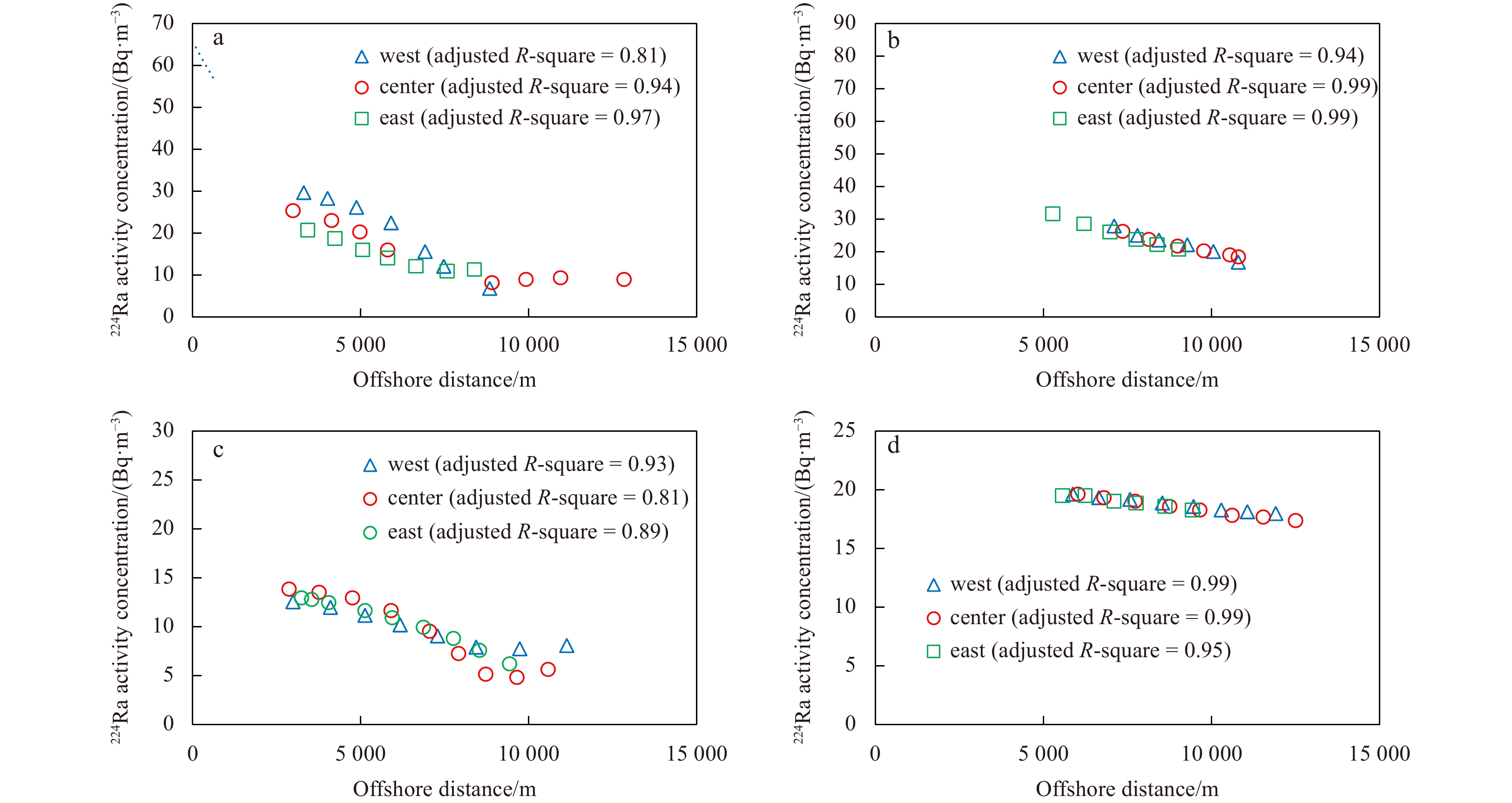
The planar distribution of 224Ra activity concentration in surface seawater can be obtained by interpolating the field data of each sampling stations (Fig. 5). Then, setting the average low tide line as the starting point (the horizontal white dash lines in Fig. 5), three transects in the offshore direction were made along the 108.52°E (west), 108.54°E (center) and 108.56°E (east) longitude respectively, and the 224Ra activity concentrations along the transects were read (the longitudinal white dash lines in Fig. 5). Thus, three groups of one-dimensional data of 224Ra longitudinal distribution of surface seawater (hereinafter referred to as one-dimensional data) can be obtained for each sampling period (Fig. 8). We assume the data obey the distribution described in Eq. (17).

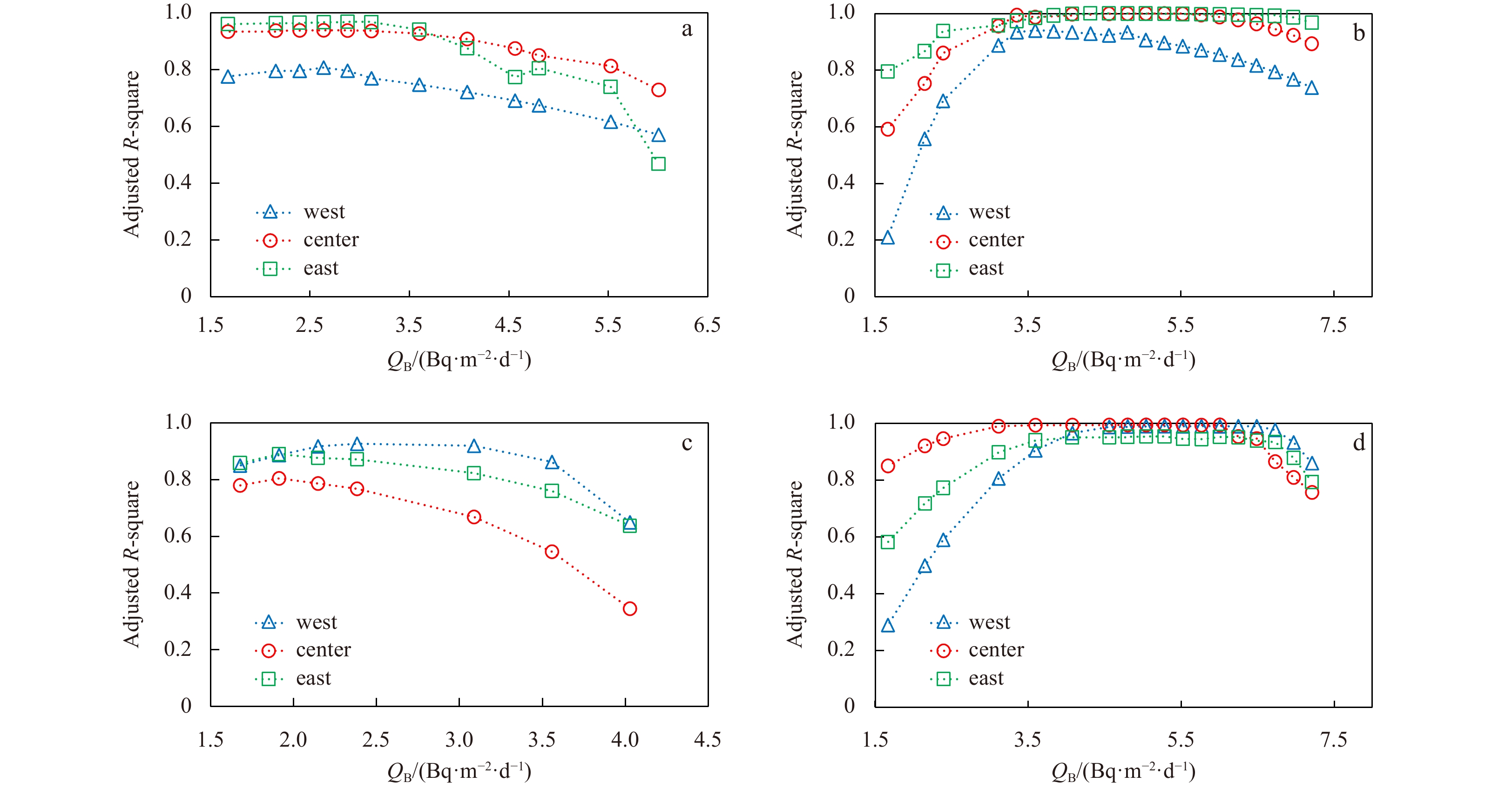
Parameter values of QB, AC_0, DL, u in Eq. (17) are undetermined at present, and the value of parameter QB needs to be determined first. For each sampling period, the one-dimensional data of 224Ra activity concentration in surface water were used to fit Eq. (17) preliminarily. In this case, it is only necessary to keep the fitting results of parameters AC_0, DL, u within a certain reasonable range, without obtaining the specific values. Assign different values to parameter QB and evaluate the quality of the corresponding fitting results by the adjusted R-square. The value is closer to “1”, the better the fitting result is. For each set of data, the QB corresponding to the best fitting effect will be accepted. The fitting results are shown in Fig. 9 and the best values of QB for each group of data are listed in Table 4.

| Parameter | Position | Sampling time | |||
| June 2016 | March 2017 | January 2019 | May 2019 | ||
| Salinity | – | 7.3 | 21.8 | 20.4 | 12.8 |
| Kd/(cm3·g–1) | – | 115.1 | 38.5 | 41.2 | 65.6 |
| Csw/(m–3) | – | 7.9×10⁶ | 1.1×10⁷ | 4.7×10⁶ | 8.8×10⁶ |
| Kz/(m·s−1) | west | 1.4×10⁻³ | 1.8×10⁻³ | 1.2×10⁻³ | 2.9×10⁻³ |
| center | 1.4×10⁻³ | 2.8×10⁻³ | 9.0×10⁻⁴ | 3.0×10⁻³ | |
| east | 1.5×10⁻³ | 2.2×10⁻³ | 9.0×10⁻⁴ | 3.0×10⁻³ | |
| Dt0/(m2·s−1) | west | 8.4×10⁻¹² | 1.4×10⁻¹¹ | 6.2×10⁻¹² | 3.6×10⁻¹¹ |
| center | 8.4×10⁻¹² | 3.4×10⁻¹¹ | 3.5×10⁻¹² | 3.9×10⁻¹¹ | |
| east | 9.6×10⁻¹² | 2.1×10⁻¹² | 3.5×10⁻¹² | 3.9×10⁻¹¹ | |
| Dw0/(m2·s−1) | west | 4.7×10⁻⁹ | 7.7×10⁻⁹ | 3.4×10⁻⁹ | 2.0×10⁻⁸ |
| center | 4.7×10⁻⁹ | 1.9×10⁻⁸ | 1.9×10⁻⁹ | 2.1×10⁻⁸ | |
| east | 5.3×10⁻⁹ | 1.2×10⁻⁸ | 1.9×10⁻⁹ | 2.1×10⁻⁸ | |
| QB/(Bq·m−2·d−1) | west | 2.8 | 3.6 | 2.5 | 5.8 |
| center | 2.8 | 5.1 | 1.9 | 6.0 | |
| east | 3.0 | 4.3 | 1.9 | 6.0 | |
| QB_st/(Bq·m−2·d−1) | west | 2.6 | 3.5 | 2.3 | 5.7 |
| center | 2.6 | 5.0 | 1.6 | 5.9 | |
| east | 2.8 | 4.1 | 1.6 | 5.9 | |
| Fst/(m3·m–1·d−1) | west | 6.3×10³ | 1.7×10⁴ | 7.4×10³ | 3.1×10⁴ |
| center | 6.3×10³ | 2.0×10⁴ | 4.2×10³ | 2.9×10⁴ | |
| east | 7.2×10³ | 1.2×10⁴ | 4.2×10³ | 2.9×10⁴ | |
| Note: Kd is solid-liquid partition coefficient; Csw is 224Ra atom quantity concentration; Kz is vertical hydraulic conductivity of seafloor sediments; Dt0 is turbulent diffusion caused by tides; Dw0 is turbulent diffusion caused by wind waves; QB is Ra flux released from bottom sediments to overlying water; QB_st is the component of QB derived by tides and waves; Fst is the single-wide flux of submarine fresh groundwater discharge. | |||||
DownLoad:
CSV
The Kz values of bottom sediment can be determined according to the discussion in Section 3.2. The turbulent diffusion coefficient driven by waves in bottom porewater and the subtidal RSGD flux (Fst, m3/(m·d)) during different periods can be determined according to Eqs (1)–(12). Parameters required for calculation are listed in Tables 3 and 4. The results are shown in Table 4.
Then, the one-dimensional data of 224Ra activity concentration in surface water were used to fit Eq. (17) for the second time to determine parameters AC_0, DL and u. The best fitting results are shown in Fig. 8. Here, all the parameters required have been determined. Finally, the Ff and Ftf can be calculated according to Eqs (22) and (23), respectively. The parameters required for calculation are listed in Table 5 and the results are shown in Table 6.
| Parameter | Position | Sampling time | |||
| June 2016 | March 2017 | January 2019 | May 2019 | ||
| AC_f/(Bq·m−3) | − | 35.0 | 23.6 | 15.5 | 11.2 |
| AC_pw/(Bq·m−3) | – | 524.4 | 498.0 | 484.4 | 279.4 |
| AC_riv/(Bq·m−3) | – | 3.1 | 3.6 | 11.2 | 12.3 |
| *AC_0/(Bq·m–3) | west | 63.2 | 64.5 | 17.1 | 21.8 |
| center | 50.0 | 74.6 | 27.0 | 22.2 | |
| east | 40.4 | 75.7 | 21.1 | 21.9 | |
| AC_SPM/(Bq·g−1) | – | 0.062 | 0.062 | 0.062 | 0.062 |
| CSPM/(g·m−3) | – | 22.4 | 14.6 | 14.6 | 22.4 |
| $\eta $ | – | 0.3 | 0.3 | 0.3 | 0.3 |
| h/m | – | 2.5 | 2.5 | 2.5 | 2.5 |
| L/m | – | 1.3×10⁴ | 1.3×10⁴ | 1.3×10⁴ | 1.3×10⁴ |
| $\text{λ} $/s–1 | – | 2.17×10⁻⁶ | 2.17×10⁻⁶ | 2.17×10⁻⁶ | 2.17×10⁻⁶ |
| (P–E)/(mm·d−1) | – | 5.5 | −1.1 | −1.6 | 2.6 |
| Friv/(m3·m–1·d−1) | – | 172.8 | 29.3 | 21.1 | 111.4 |
| *u/(m·s−1) | west | 5.9×10⁻³ | 1.0×10⁻³ | 6.1×10⁻⁴ | 3.5×10⁻³ |
| center | 5.8×10⁻³ | 1.0×10⁻³ | 5.8×10⁻⁴ | 3.5×10⁻³ | |
| east | 5.9×10⁻³ | 1.0×10⁻³ | 6.5×10⁻⁴ | 3.5×10⁻³ | |
| *DL/(m·s−2) | west | 10.2 | 57.6 | 96.8 | 1073.0 |
| center | 10.0 | 42.1 | 28.5 | 720.8 | |
| east | 10.4 | 37.8 | 52.5 | 834.5 | |
| Note: AC_f is the 224Ra activity concentration of fresh groundwater end member; AC_pw is the 224Ra activity concentration of porewater end member; AC_riv is the 224Ra activity concentration of river water; *AC_0 is the 224Ra activity concentration of water in the land-sea boundary; AC_SPM is the 228Th activity of per unit mass sediment; CSPM is the mass concentration of suspended particulate matter in seawater; r in seawater; $\eta $ is maximum desorption ratio of Ra on the suspended particulate matter; h is the mean water depth; L is the spatial scale of the study water area; $ \text{λ} $ is the decay constant of 224Ra; P and E represent precipitation and evaporation in the study area, respectively; Friv is the surface runoff; *u is mean offshore velocity; *DL is turbulent diffusion coefficient of coastal water. The parameters labeled with * were obtained by fitting Eq. (17) with experimental data. AVG: average value. | |||||
DownLoad:
CSV
| Items | Position | Sampling time | |||
| June 2016 | March 2017 | January 2019 | May 2019 | ||
| Ff/(m3·m−1·d−1) | west | 132.2 | 115.6 | 62.4 | 85.5 |
| center | 211.4 | 35.0 | 36.1 | 95.7 | |
| east | 146.4 | 116.3 | 89.0 | 107.8 | |
| AVG | 163.3 | 89.0 | 62.5 | 163.3 | |
| Ftf/(m3·m−1·d−1) | west | 580.8 | 445.6 | 80.1 | 321.0 |
| center | 401.6 | 367.7 | 94.4 | 279.0 | |
| east | 307.9 | 351.7 | 79.7 | 254.6 | |
| AVG | 430.0 | 388.3 | 84.7 | 430.0 | |
| Note: Ff is the single-wide flux of SFGD; Ftf is the single-wide exchange capacity of tidal flat RSGD. AVG: average value. | |||||
DownLoad:
CSV
The width of the Maowei Sea is about 15 km, and the water area is about 135 km2 (He, 2015). Given the single wide fluxes of these components of SGD, the average daily flows of these components for the whole area can be obtained. For comparison, the single wide fluxes and the daily flows for the whole area of all the SGD components are plotted in Fig. 10.

The single wide flux of SFGD in the Maowei Sea is on the order of 1×10² m3/(m·d), which is slightly lower than that of tidal flat RSGD, but these two are on the same order of magnitude. The single wide flux of subtidal RSGD is on the order of 1×10⁴ m3/(m·d) which is significantly higher than the other two components. The average daily flows of SFGD and tidal flat RSGD along the coastline are all on the order of 1×10⁵ m3/d, and the latter is slightly higher than the former. As for subtidal RSGD, the average daily flow is on the magnitude of 1×10⁶–1×10⁷ m3/d. It can be concluded that the extensive subtidal zone takes an important role in the total flux of RSGD. In the studies of SGD and its impact on the coastal environment, it is necessary to distinguish the different components of SGD in addition to estimating the total average SGD flux for the whole area. In general, SFGD contributes net freshwater flows to coastal water while carrying terrigenous materials into the sea. Tidal flat RSGD promotes the water circulation and material exchange between coastal water body and aquifer. As for subtidal RSGD, it leads to the water circulation and material exchange between the bottom porewater and the overlying water. The origins of the three components of SGD are different, so as the chemical constituents. Therefore, the effects of different SGD components on coastal environment are also different, which should be considered separately.
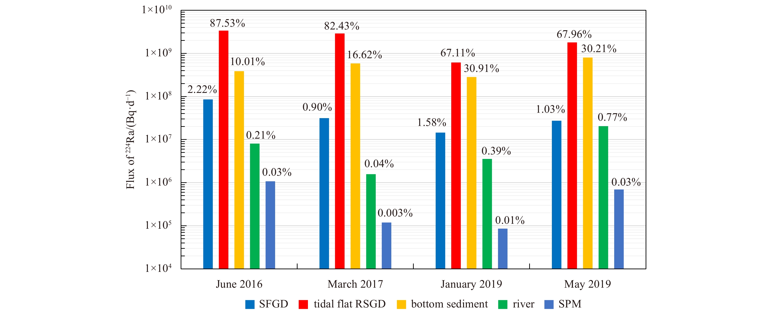
Finally, the contribution of each source item to 224Ra in the Maowei Sea waterbody was calculated (Fig. 11). In general, the average 224Ra activity flux contributed by tidal flat RSGD, subtidal RSGD and SFGD are about 2.18×10⁹ Bq/d, 5.14×10⁸ Bq/d and 3.98×10⁷ Bq/d, respectively. Among all types of 224Ra sources, tidal flat RSGD accounted for the highest proportion, reaching 76.3%; subtidal RSGD accounts for 30%, ranking second; SFGD accounted for only 1.4%; riverine sources contribute less than 1%.

Researchers are more interested in the tidal flat RSGD and SFGD for purpose of better understanding of the land-sea interactions and the effects of terrigenous materials on coastal ecosystems. For a certain study area, compared with the SGD flux in a certain period, the long-term variation trend of SGD is more valuable information. In this section, based on Ra tracing method, a relatively simple and reliable method is built to realize the long-term monitoring of SGD fluxes with lower cost.
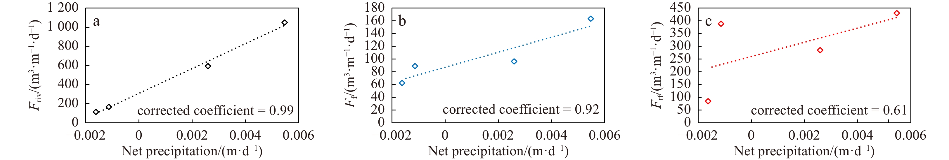
Taking time as an independent variable is a natural and intuitive idea. However, the SGD fluxes generally show periodically variations over time (Wilson et al., 2015). It is difficult to accurately predict the periodic variations with small amounts of field data, so time is not suitable as an independent variable. For a certain study area, the precipitation and evaporation also show periodic variations over time. Researches show that the groundwater table is approximately linearly related to regional precipitation (Liu and Wang, 2009; Zhang et al., 2008), and the groundwater table variation may have influence on the RSGD flux (Robinson, et al., 2007; Yu, 2021). More importantly, the relationship between the above variables is mutually monotonous. In view of this, we select net precipitation as the independent variable in this study, which is more appropriate in condition of small amounts of field data. In the following, the relations between net precipitation and the fluxes of SFGD and tidal flat RSGD in the Maowei Sea were explored. The precipitation and evaporation data in study area are available on the National Center for Environmental Information (NCEI) website (
| $$ {P}_{{\rm{n}}}=P-E . $$ | (24) |
Taking Pn as the independent variable, the relationships between Pn and surface runoff, as well as the fluxes of SFGD and tidal flat RSGD are plotted in Fig. 12.

It can be seen that both surface runoff and SFGD flux have a good linear correlation with net precipitation. For simplicity, linear functions are adopted to fit the relationships between the former two and net precipitation respectively:
| $$ {F}_{{\rm{riv}}}={K}_{{\rm{r}}0}{P}_{{\rm{n}}}+{F}_{{\rm{r}}0} , $$ | (25) |
| $$ {F}_{{\rm{f}}}={K}_{{\rm{f}}0}{P}_{{\rm{n}}}+{F}_{{\rm{f}}0} , $$ | (26) |
where the coefficients Kr0 (1.30×10⁵ m) and Kf0 (1.18×10⁴ m) represent the increment of surface runoff or tidal flat SFGD flux caused by an increase of one unit of net precipitation respectively. The coefficients Fr0 (308.4 m3/(m·d)) and Ff0 (87.2 m3/(m·d)) represent the surface runoff or SFGD flux when the net precipitation is zero.
Substitute Eqs (19), (25) and (26) into Eq. (22), after simplification, the expression of tidal flat RSGD flux with net precipitation as independent variable can be expressed as follows:
| $$\tag{27a} {F}_{{\rm{tf}}}={a}_{1}{P}_{{\rm{n}}}+{c}_{1}+{b}_{1}\sqrt{{a}_{2}{P}_{{\rm{n}}}^{2}+{b}_{2}{P}_{{\rm{n}}}+{c}_{2}} , $$ |
where the expression of each coefficient is
| $$\tag{27b} \begin{split}{a}_{1}=&\dfrac{1}{2\text{λ} \left({A}_{{\rm{C}}\_0}-{A}_{{\rm{C}}\_{\rm{pw}}}\right)}\Bigg[-\left({Q}_{{\rm{B}}}+\text{λ} h{A}_{{\rm{C}}\_0}\right)\left(\dfrac{{K}_{{\rm{f}}0}+{K}_{{\rm{r}}0}}{h}+\dfrac{L}{2h}\right)+\\ &2\text{λ} \left({K}_{{\rm{f}}0}{A}_{{\rm{C}}\_{\rm{f}}}+{{{K}}}_{{\rm{r}}0}{A}_{{{{\rm{C}}}}\_{\rm{riv}}}+{{{{C}}}_{{\rm{SPM}}}{A}_{{\rm{C}}\_{\rm{SPM}}}\eta K}_{{\rm{f}}0}\right)\Bigg] ,\\[-18pt]\end{split} $$ |
| $$\tag{27c} {b}_{1}=\frac{{Q}_{{\rm{B}}}-\text{λ} h{A}_{{\rm{C}}\_0}}{2\text{λ} \left({A}_{{\rm{C}}\_0}-{A}_{{\rm{C}}\_{\rm{pw}}}\right)} , $$ |
| $$\tag{27d} \begin{split} {c}_{1}=&\dfrac{1}{2\text{λ} \left({A}_{{\rm{C}}\_0}-{A}_{{\rm{C}}\_{\rm{pw}}}\right)}\Bigg[2\text{λ} ({F}_{{\rm{f}}0}{A}_{{\rm{C}}\_{\rm{f}}}+{F}_{{\rm{r}}0}{A}_{{\rm{C}}\_{\rm{riv}}}+\\&{C}_{{\rm{SPM}}}{A}_{{\rm{C}}\_{\rm{SPM}}}\eta {F}_{{\rm{f}}0})-{A}_{{{\rm{C}}}_{0}}\left({F}_{{\rm{f}}0}+{F}_{{\rm{r}}0}\right)-\dfrac{{Q}_{{\rm{B}}}\left({F}_{{\rm{f}}0}+{F}_{{\rm{r}}0}\right)}{h}\Bigg] ,\end{split} $$ |
| $$\tag{27e} {a}_{2}={\left(\frac{{K}_{{\rm{f}}0}+{K}_{{\rm{r}}0}}{h}+\frac{L}{2h}\right)}^{2} , $$ |
| $$\tag{27f} {b}_{2}=2\left({F}_{{\rm{f}}0}+{F}_{{\rm{r}}0}\right)\left(\frac{{K}_{{\rm{f}}0}+{K}_{{\rm{r}}0}}{h}+\frac{L}{2h}\right) , $$ |
| $$\tag{27g} {c}_{2}=\frac{{\left({F}_{{\rm{f}}0}+{F}_{{\rm{r}}0}\right)}^{2}}{h}+4{\text{λ} D}_{{\rm{f}}0} . $$ |
In general, Eq. (27) can be regarded as the addition of a linear function (the first two terms on the right) and a nonlinear function (the third term on the right). It should be noted that, although the coefficients in Eq. (27) contain physical quantities related to 224Ra concentration and its transport process, these physical quantities are not the essential factors determining the tidal flat RSGD flux, but only play a “representation” role. The factors that are intrinsically related to the RSGD flux are hydrogeological or meteorological factors such as the coastal aquifer properties, land-seawater force gradient variations, precipitation and evaporation, etc. In order to explore the variation trend of tidal flat RSGD flux with net precipitation under different conditions, sensitivity analysis is needed. The parameters in Eq. (27) were assigned certain values with reference to existing field data, and the net precipitation was set within a certain range (−1–5 mm/d). Taking surface runoff as a reference, by changing the relative value of SFGD flux to surface runoff, the response of tidal flat RSGD flux to the net precipitation under different SFGD flux conditions was calculated. The parameters required are listed in Table 7.
| Parameter | Value | |||||
| h/m | 2.5 | |||||
| L/m | 13000 | |||||
| DL/(m2·s−1) | 100 | |||||
| QB/(Bq·m–2·d−1) | 3 | |||||
| AC_0/(Bq·m−3) | 30 | |||||
| AC_f/(Bq·m−3) | 50 | |||||
| AC_pw/(Bq·m−3) | 500 | |||||
| AC_riv/(Bq·m−3) | 10 | |||||
| AC_SPM/(Bq·m−3) | 0.062 | |||||
| CSPM/(g·m−3) | 25 | |||||
| $\eta $ | 0.3 | |||||
| Kr0/m | 1×10⁵ | |||||
| Fr0/(m3·m−1·d−1) | 100 | |||||
| Kf0/m | 5×10³ | 1×10⁴ | 3×10⁴ | 7×10⁴ | 1×10⁵ | 1.2×10⁵ |
| Ff0/(m3·m–1·d–1) | 5 | 10 | 30 | 70 | 100 | 120 |
| Note: h is the mean water depth; L is the spatial scale of the study water area; DL is turbulent diffusion coefficient of coastal water. QB is Ra flux released from bottom sediments to overlying water; AC_0 is the 224Ra activity concentration of water in the land-sea boundary; AC_f is the 224Ra activity concentration of fresh groundwater endmember; AC_pw is the 224Ra activity concentration of porewater endmember; AC_riv is the 224Ra activity concentration of river water; AC_SPM is the 228Th activity of per unit mass suspended particulate matter; CSPM is the mass concentration of suspended particulate matter in seawater; $ \eta$ is maximum desorption ratio of Ra on the suspended particulate matter; Kr0 and Kf0 represent the increment of surface runoff or tidal flat submarine fresh groundwater discharge (SFGD) flux caused by an increase of one unit of net precipitation respectively; Fr0 and Ff0 represent the surface runoff or SFGD flux when the net precipitation is zero. | ||||||
DownLoad:
CSV
The results of sensitivity analysis are shown in Fig. 13. When the ratio of SFGD flux to surface runoff is small (in this study, the ratio less than 0.3), the linear component of Ftf show a positive linear correlation with net precipitation. When the ratio becomes higher (in this study, the ratio larger than 0.7), the linear component shows a negative linear correlation of net precipitation (Fig. 13). Regardless of the relative scale of SFGD flux versus surface runoff, the nonlinear components of Ftf always increase with the increase of net precipitation. Under the condition of the same net precipitation, the higher the SFGD flux, the higher the nonlinear component of Ftf (Fig. 13). Under the conditions of different net precipitation, the absolute values of the nonlinear and linear components of Ftf are basically on the same order of magnitude. The maximum of the ratio of the two components only occurs in case of relatively higher SFGD flux together with higher net precipitation, and this is due to the zero value of linear component of Ftf on the above condition. The overall variation trend of Ftf can be obtained by adding the linear and nonlinear components. As can be seen from Fig. 13d that the overall variation trend of Ftf is similar to that of the linear component.

The results of the above sensitivity analysis can be explained qualitatively as follows: the SGD flux is positively correlated with the land-sea hydraulic gradient (Lee et al, 2013; Yu, 2021). The lower SFGD flux represents smaller land-sea hydraulic gradient which becomes the limiting condition for the tidal flat RSGD flux. With the increase of net precipitation, the water level of aquifer will be raised, and the land-sea hydraulic gradient also increases. As a result, the RSGD flux will increase correspondingly. In the case of relatively higher SFGD flux, the land-sea hydraulic gradient is no longer a limiting condition. At this time, the increase of net precipitation will promote SFGD flux. The strong seaward fresh groundwater flow will push the wave-induced circulation zone to the offshore direction, thus limiting the scale of tidal flat RSGD flux (Robinson et al., 2007).
According to the discussion above, although the expression of tidal flat RSGD (Eq. (27)) contains nonlinear components, its overall trend is still close to linear function (Fig. 13d). The tidal flat RSGD flux in the Maowei Sea based on the field data is approximately linearly positive correlated with the net precipitation during the sampling period (corrected coefficient = 0.61). Therefore, linear function is still adopted to describe the relationship between tidal flat RSGD flux and net precipitation in the Maowei Sea:
| $$ {F}_{{\rm{tf}}}={K}_{{\rm{t}}0}{P}_{{\rm{n}}}+{F}_{{\rm{t}}0} , $$ | (28) |
where coefficient Kt0 (2.79×10⁴ m) represents the increment in tidal flat RFGD flux for each unit increase in net precipitation. Ft0 (260.0 m3/(m·d)) represents the tidal flat RSGD flux corresponding to zero net precipitation.
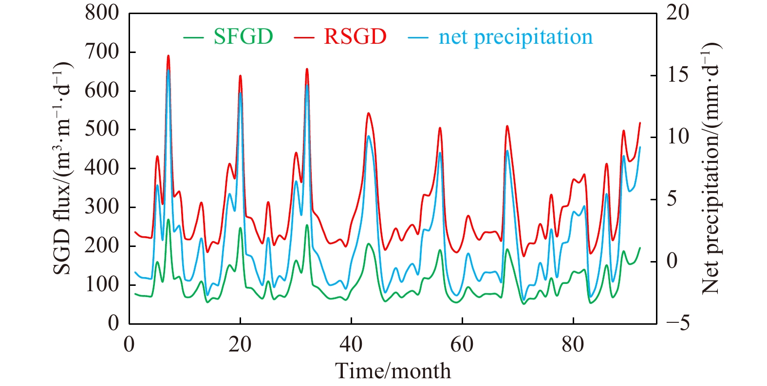
As an application example, we select January 2015 to August 2022 as the study period to calculate the fluxes of SFGD and tidal RSGD according to Eqs (26) and (28) respectively. The precipitation and evaporation data were obtained from the NCEI website of NOAA (

In this section, we will compare the results of this study with the existing relevant studies. The comparison is mainly made in two aspects: (1) separating the SGD components, and (2) the long-term variation trend of SGD.
There already have some studies related to the differentiation of SGD components worldwide. This section gives a brief overview and compares them with the results of this study (Table 8). The seepage meter combined with water salinity is one of the common methods for separating SGD components. Taniguchi et al. (2008b) choose the Flamengo Bay located near the city of Ubatuba, Sao Paulo State, Brazil as the study area. The SGD flux below the low water line was measured with seepage meters and SFGD components were distinguished by water and salinity conservation. The SGD fluxes at 10 m, 40 m and 50 m distance offshore from the low tide mark were estimated to be 2.6 m/d, 0.038 m/d and 1.86 m/d, respectively. And the SFGD accounted for 5.5%, 5.1% and 24.7% in the SGD, respectively. Similarly, Taniguchi et al. (2008a) estimated the SGD fluxes from the Huanghe River Delta to the Bohai Sea with seepage meters, and distinguished SFGD components by water and salinity conservation. The mean SGD fluxes in September 2004, May 2005 and September 2006 were estimated to be 8.04×10⁸ m3/d, 1.04×10⁸ m3/d and 1.73×10⁸ m3/d, respectively. The total SGD were found to be 13.8, 8.5 and 16.0 times the river discharge into the Bohai Sea. The SFGD fluxes in September 2004 and September 2006 were estimated to be 9.5×10⁶ m3/d and 1.47×10⁷ m3/d, accounting for 1.18% and 8.47% of the total SGD in the same period.
It is also feasible to distinguish the SGD components by natural traces. Zhang et al. (2018) estimated the SGD flux in the North Liaodong Bay, Bohai Sea, China. And separated the SFGD and RSGD components using Ra, water and salt balance model. The SGD flux was estimated to be 1.48×10⁸ −5.96×10⁸ m3/d, while the SFGD flux was about 5.79×10⁷−6.66×10⁷ m3/d, accounting for 11.17%−18.85% of the total SGD. Liu et al. (2021) used 226Ra and 228Ra as tracers to estimate the SGD flux and separate SFGD from RSGD in the Yellow Sea by establishing a double-end-member model. The average flux of SGD was estimated to be 2.14×10⁹−8.49×10⁹ m3/d, of which SFGD accounted for 5.2%−8.8%.
Li and Jiao (2013) summarized the existing SGD related studies and found that the SGD flux estimated by the hydrological model method was at least one order of magnitude different from that estimated by the isotope tracer method. One of the possible reasons is that the spatial scale of the hydrological model method is limited to inland or near the intertidal zone, and the submarine groundwater-overlying water circulation in the wide intertidal zone below the low tide line may be ignored Post et al. (2013). Huang (2015) and Ma (2016) established a hydrological model of subtidal groundwater-overlying water circulation and proposed an analytical solution. Ma (2016) selected a tidal flat in the south of the Laizhou Bay, Bohai Sea, China as the study area, and estimated the tidal flat SGD flux of 4.95 m3/(m·d) by combining the field data with the numerical model. The SFGD flux was about 0.26 m3/(m·d), accounting for about 5% of the tidal flat SGD. The subtidal RSGD exchange capacity is 104 m3/(m·d), which is much higher than the tidal flat SGD flux.
| Study area | Method or tracer | Date | Distance offshore from the low tide mark/m | Result | Reference | ||
| SGD | SFGD | RSGD | |||||
| Flamengo Bay near the city of Ubatuba, Sao Paulo State | seepage meter | Nov. 2003 | 10 | 2.6 m/d | 0.14 m/d | − | Taniguchi et al. (2008b) |
| 40 | 0.038 m/d | 2×10⁻³ m/d | − | Taniguchi et al. (2008b) | |||
| 50 | 1.86 m/d | 0.46 m/d | − | Taniguchi et al. (2008b) | |||
| Huanghe River Delta | seepage meter | Sept. 2004 | − | 8.04×10⁸ m3/d | 9.50×10⁶ m3/d | − | Taniguchi et al. (2008a) |
| May 2005 | − | 1.04×10⁸ m3/d | − | − | Taniguchi et al. (2008a) | ||
| Sept. 2006 | − | 1.73×10⁸ m3/d | 1.47×10⁷ m3/d | − | Taniguchi et al. (2008a) | ||
| North Liaodong Bay, Bohai Sea, China | Ra, water and salt balance model | Apr. and May 2017 | − | 1.48×10⁸−5.96× 10⁸ m3/d | 5.79×10⁷−6.66× 10⁷ m3/d | − | Zhang (2018) |
| Yellow Sea | 226Ra and 228Ra | Apr. and May 2014 | − | 2.14×10⁹−8.49× 10⁹ m3/d | 1.64×10⁷−11.2× 10⁷ m3/d | − | Liu et al. (2021) |
| Laizhou Bay, Bohai Sea | hydrological model | Sept. 2012 | − | − | 0.26 m3/(m·d) | 4.95 m3/(m·d)a, 1×10⁴ m3/(m·d)b | this study |
| Maowei Sea, Guangxi, China | 224Ra | Jun. 2016 | − | − | 163.33 m3/(m·d) | 430.09 m3/(m·d)a, 6.59×10³ m3/(m·d)b | this study |
| Mar. 2017 | − | − | 88.97 | 388.32 m3/(m·d)a, 1.64×10⁴ m3/(m·d)b | this study | ||
| Jan. 2019 | − | − | 62.48 | 84.73 m3/(m·d)a, 5.23×10³ m3/(m·d)b | this study | ||
| May 2015 | − | − | 163.33 | 430.09 m3/(m·d)a, 2.95×10⁴ m3/(m·d)b | this study | ||
| Note: SGD: submarine groundwater discharge; SFGD: submarine fresh groundwater discharge; RSGD: recirculated saline groundwater discharge; superscript a represents tidal flat RSGD; superscript b represents subtidal RSGD. − represents no data. | |||||||
DownLoad:
CSV
The units of SGD fluxes derived from different studies are different. For the convenience of comparison, the unit here is unified as “m3/(m2·d)”. The study areas of Huanghe River Delta, Liaodong Bay, Yellow Sea and Maowei Sea are 2.50×10¹¹ m2 (Taniguchi et al., 2008a), 9.50×10⁹ m2 (Zhang, 2018), 4.00×10¹¹ m2 (Liu et al., 2021) and 1.35×10⁸ m2 (Chen, 2019), respectively. In conclusion, the average SGD fluxes in Huanghe River Delta, Liaodong Bay, Yellow Sea and Maowei Sea are estimated to be about 1.44×10⁻³ m3/(m2·d), 3.92×10⁻² m3/(m2·d), 1.33×10⁻² m3/(m2·d) and 4.80×10⁻² m3/(m2·d). The average fluxes of SFGD are estimated to be about 4.84×10⁻⁵ m3/(m2·d), 6.55×10⁻³ m3/(m2·d), 1.61×10⁻⁴ m3/(m2·d) and 4.76×10⁻⁴ m3/(m2·d). By comparison, it can be concluded that the total SGD flux in the Maowei Sea is at a relatively high level and the SFGD flux is at a moderate level in all coastal regions of China.
There have been abundant studies on the long-term variation trend of SGD. Seasonal variations of the 226Ra activities observed by Moore (2007, 2010b) along the transect of Winyah Bay, South Atlantic Bight, indicate that the SGD is very large (in the order of 1000 m3/(m·d) in summer but close to zero in winter and spring. Zhang et al. (2017) analyzed the monthly groundwater level of the Toyama Bay in central Japan in recent 30 years by using monthly precipitation, monthly snowfall and climate change index. The results show that the regional rainfall has been on the rise in the past 40 years, and the SGD flux estimated from the change of groundwater level also shows an upward trend. The regional SGD flux is of the order of 6×10⁷ m3/a (1.64×10⁵ m3/d), which is about 20% of river discharge. Considering the continuous increase of regional precipitation, it is predicted that regional SGD will reach 7×10⁷ m3/a and 8×10⁷ m3/a in 2030 and 2050, respectively. Hsu et al. (2020) adopted natural tracers (222Rn, 224Ra, 228Ra, δD and δ18O) to conducted time series observations of SGD flux in the Gaomei wetland south of the mouth of the Taiga River in western Taiwan Island. The results showed that SGD flux varied with tidal changes. The SGD fluxes in dry season and wet season were (0.002−0.25) m/d and (0.001−0.47) m/d, respectively. The SGD flux was slightly higher during the spring tide in the rainy season, indicating that the tidal pumping was stronger and the gradient of sea-land water potential was larger. The variation of SGD in the Gaomei wetland is controlled not only by the seasonal change of groundwater recharge, but also by the tidal pumping process.
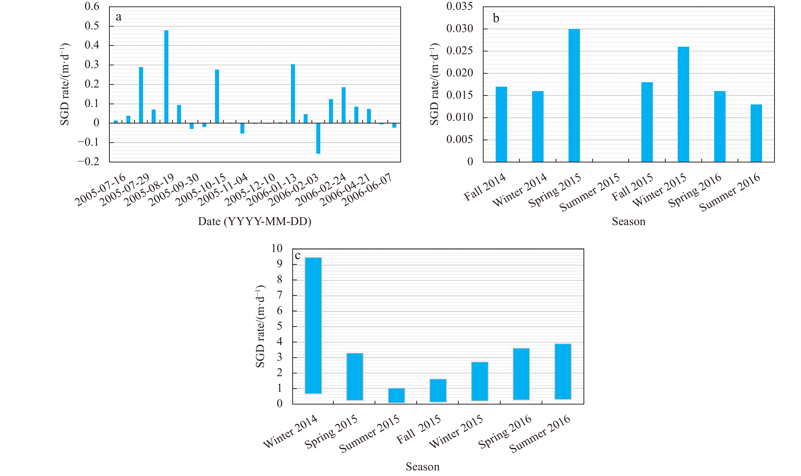
It seems that SGD is basically positively correlated with precipitation, which is similar to the result of this study. However, there are still some special conditions. Uddameri et al. (2014) conducted a one-year survey of submarine groundwater discharge at Loyola Beach, Baffin Bay, Texas, from July 2005 to June 2006 (Fig. 15a). A total of 23 weather-related SGD sampling events were conducted, most of which used an ultrasonic penetrator to collect SGD data continuously for 24 h at a time resolution of 1 min. The median SGD was 3.83 cm/d, and the interquartile distance (IQR) was 11.36 cm/d. The proportion of SFGD to SGD was estimated to vary between 4% and 89%, with a median of 9.96% and an IQR of 7.16%. Four sampling events had anomalously high SGD values ((27–48) cm/d) and three events were noted to have abnormally high SFGD fractions (28%, 50% and 84%) which are likely artifacts caused by bay water freshening from rainfall and plausible thermal expansion. Short-term diurnal variability of SGD is comparable to, and sometimes even higher than long-term and interevent variability. Long-term variation trends of SGD in this region cannot be inferred. Murgulet et al. (2018) and Douglas et al. (2020) selected semi-arid, weakly tidal and human-disturbed estuary, the Gulf of Mexico and Nueces River basin of Texas, the United States, as study area. By using the Darcy’s law and mass balance method of 222Rn and 226Ra, the spatial-temporal variation of SGD under different hydroclimatic conditions is studied. The range of SGD flux estimated by Darcy’s law is (0.09−8.28) m/d, and the SGD flux estimated by 226Ra and 222Rn are shown in Figs 15b and c. The results suggest that changes in semi-arid, highly human-disturbed groundwater systems may lag climatic conditions by weeks (shallow aquifers) or months or longer (deep aquifers).

In summary, studies related to SGD are complicated due to the influence of geology, climate and human activities. Different study area has its own pattern characteristics. For a certain area, a personalized and specific research scheme should be formulated to find out the main factors affecting SGD on the basis of sufficient field data, and an appropriate model should be adopted to describe the variation trend of SGD according to the characteristics of the region.
In this study, the three main components of SGD (SFGD, tidal flat RSGD, subtidal RSGD) in the Maowei Sea were distinguished and their corresponding fluxes were also estimated based on the field data with 224Ra as the tracer. The conclusions of this study can be summarized as follows:
(1) In general, the average daily flow along the coastline of the Maowei Sea of tidal flat RSGD is slightly higher than that of SFGD, and both are on the magnitude of 1×10⁵ m3/d. However, the average daily flow of subtidal RSGD of the entire subtidal zone of the Maowei Sea reaches the magnitude of 1×10⁶−1×10⁷ m3/d, which is significantly higher than the first two. It can be concluded that the circulation driven by waves between the bottom sediment and overlying water in wide subtidal zone play a main role in the total RSGD flux for the study area. Compared with previous, it can be concluded that the total SGD flux in the Maowei Sea is at a relatively high level and the SFGD flux is at a moderate level in all coastal regions of China.
(2) For a certain study area, the permeability of bottom sediment has a significant influence on the subtidal RSGD flux. The results of sensitivity analysis showed that in condition of the value of Kz exceeds 1×10⁻³ m/s, 224Ra flux carried by subtidal RSGD accounts for more than 90% of the total 224Ra flux released by bottom sediment to overlying water. For the subtidal zone of the Maowei Sea, the average value of Kz is about 1.9 × 10⁻³ m/s which is significantly higher than typical values for terrestrial aquifer. The average flux of 224Ra released by bottom sediment in the subtidal zone of the Maowei Sea is about 3.7 Bq/(m2·d), and the proportion of subtidal RSGD contribution reached 97.8%. Among all the sources of 224Ra in the Maowei Sea, the contribution of bottom sediments accounts for about 21.9%, second only to tidal flat RSGD (76.3%).
(3) Through the analysis of the results of SGD in four different periods in the Maowei Sea, it is found that the fluxes of SFGD and tidal flat RSGD all have a good positive linear correlation with regional net precipitation. The net precipitation can be selected as an independent variable, and the variation trends of SFGD as well as tidal flat RSGD can be described by linear function respectively. The net precipitation data of the Maowei Sea from January 2015 to August 2022 were adopted to calculate the regional fluxes of SFGD and tidal flat RSGD. It is concluded that the flux of subtidal RSGD is slightly higher than that of SFGD overall, and the differences between the two is larger in the flood season while smaller in the dry season. SGD trends in many regions are positively correlated with precipitation, which is similar to the results of this study. However, there are some exceptions. The influencing factors of SGD are complex and different study areas have unique situations. Specific research schemes should be formulated according to the local characteristics.
Acknowledgements: The authors thank Bin Yang of Beibu Gulf University for the help with sampling.|
Anschutz P, Smith T, Mouret A, et al. 2009. Tidal sands as biogeochemical reactors. Estuarine, Coastal and Shelf Science, 84(1): 84–90
|
|
Boehm A B, Shellenbarger G G, Paytan A. 2004. Groundwater discharge: potential association with fecal indicator bacteria in the surf zone. Environmental Science & Technology, 38(13): 3558–3566
|
|
Boudreau B P. 1996. The diffusive tortuosity of fine-grained unlithified sediments. Geochimica et Cosmochimica Acta, 60(16): 3139–3142. doi: 10.1016/0016-7037(96)00158-5
|
|
Burnett W C, Bokuniewicz H, Huettel M, et al. 2003. Groundwater and pore water inputs to the coastal zone. Biogeochemistry, 66(1–2): 3–33
|
|
Burnett W C, Taniguchi M, Oberdorfer J. 2001. Measurement and significance of the direct discharge of groundwater into the coastal zone. Journal of Sea Research, 46(2): 109–116. doi: 10.1016/S1385-1101(01)00075-2
|
|
Canuel E A, Cammer S S, McIntosh H A, et al. 2012. Climate change impacts on the organic carbon cycle at the land-ocean interface. Annual Review of Earth and Planetary Sciences, 40: 685–711. doi: 10.1146/annurev-earth-042711-105511
|
|
Charette M A, Dulaiova H, Gonneea M E, et al. 2012. GEOTRACES radium isotopes interlaboratory comparison experiment. Limnology and Oceanography: Methods, 10(6): 451–463. doi: 10.4319/lom.2012.10.451
|
|
Chen Xiaogang. 2019. Submarine groundwater discharge in mangroves, salt marshes, sandy beaches and karst ecosystems of typical coastal zones (in Chinese)[dissertation]. Shanghai: East China Normal University
|
|
Codification Committee of Gulf Records of China. 1993. Gulf Records of China, Vol. 12 (in Chinese). Beijing: China Ocean Press, 144–197
|
|
Colbert S L, Hammond D E. 2007. Temporal and spatial variability of radium in the coastal ocean and its impact on computation of nearshore cross-shelf mixing rates. Continental Shelf Research, 27(10–11): 1477–1500
|
|
Douglas A R, Murgulet D, Peterson R N. 2020. Submarine groundwater discharge in an anthropogenically disturbed, semi-arid estuary. Journal of hydrology, 580: 124369. doi: 10.1016/j.jhydrol.2019.124369
|
|
Garcia-Orellana J, Cochran J K, Bokuniewicz H, et al. 2014. Evaluation of 224Ra as a tracer for submarine groundwater discharge in Long Island Sound (NY). Geochimica et Cosmochimica Acta, 141: 314–330. doi: 10.1016/j.gca.2014.05.009
|
|
Gibbes B, Robinson C, Li L, et al. 2008. Tidally driven pore water exchange within offshore intertidal sandbanks: part Ⅱ numerical simulations. Estuarine, Coastal and Shelf Science, 80(4): 472–482
|
|
Gu Hequan. 2015. A quantitative study on the sources and sinks of radium isotopes in near-shore waters—Taking Changjiang estuary and its adjacent offshore area, Bamen Lagoon, Gaolong Bay and Boao Bay in Hainan for example (in Chinese)[dissertation]. Shanghai: East China Normal University
|
|
Hancock G J, Webster I T, Ford P W, et al. 2000. Using Ra isotopes to examine transport processes controlling benthic fluxes into a shallow estuarine lagoon. Geochimica et Cosmochimica Acta, 64(21): 3685–3699. doi: 10.1016/S0016-7037(00)00469-5
|
|
He Shuai. 2015a. Numerical study on water quality and environmental capacity of Maowei Sea (in Chinese)[dissertation]. Qingdao: Ocean University of China
|
|
He Zhengzhong. 2015b. Sedimentation rate research in Guangxi Beibu Gulf (in Chinese)[dissertation]. Nanning: Guangxi University
|
|
Hsu Feng-Hsin, Su Chih-Chieh, Wang Pei-Ling, et al. 2020. Temporal variations of submarine groundwater discharge into a tide-dominated coastal wetland (Gaomei Wetland, Western Taiwan) indicated by radon and radium isotopes. Water, 12(6): 1806. doi: 10.3390/w12061806
|
|
Huang Ya’nan. 2015. An analytical study of tidal-induced seawater-groundwater exchange rate through a horizontal seabed (in Chinese)[dissertation]. Beijing: China University of Geosciences (Beijing)
|
|
Ip C C M, Li Xiangdong, Zhang Gan, et al. 2007. Trace metal distribution in sediments of the Pearl River Estuary and the surrounding coastal area, South China. Environmental Pollution, 147(2): 311–323. doi: 10.1016/j.envpol.2006.06.028
|
|
Katz A J, Thompson A H. 1985. Fractal sandstone pores: implications for conductivity and pore formation. Physical Review Letters, 54(12): 1325–1328. doi: 10.1103/PhysRevLett.54.1325
|
|
Knauss J A. 1996. Introduction to Physical Oceanography. 2nd ed. Upper Saddle River, New Jersey: Prentice Hall, 176–201
|
|
Knee K L, Paytan A. 2011. 4.08-submarine groundwater discharge: a source of nutrients, metals, and pollutants to the coastal ocean. Treatise on Estuarine and Coastal Science, 4: 205–233
|
|
Krishnaswami S, Graustein W C, Turekian K K, et al. 1982. Radium, thorium and radioactive lead isotopes in groundwaters: application to the in situ determination of adsorption-desorption rate constants and retardation factors. Water Resources Research, 18(6): 1663–1675. doi: 10.1029/WR018i006p01663
|
|
Krohn C E, Thompson A H. 1986. Fractal sandstone pores: automated measurements using scanning-electron-microscope images. Physical Review B, 33(9): 6366–6374. doi: 10.1103/PhysRevB.33.6366
|
|
Lamontagne S, Webster I T. 2019. Cross-shelf transport of submarine groundwater discharge tracers: a sensitivity analysis. Journal of Geophysical Research: Oceans, 124(1): 453–469. doi: 10.1029/2018JC014473
|
|
Lecher A L, Kessler J, Sparrow K, et al. 2016. Methane transport through submarine groundwater discharge to the North Pacific and Arctic Ocean at two Alaskan sites. Limnology and Oceanography, 61(S1): S344–S355. doi: 10.1002/lno.10118
|
|
Lee E, Hyun Y, Lee K K. 2013. Sea level periodic change and its impact on submarine groundwater discharge rate in coastal aquifer. Estuarine, Coastal and Shelf Science, 121–122: 51–60
|
|
Li Yuanhui, Gregory S. 1974. Diffusion of ions in sea water and in deep-sea sediments. Geochimica et Cosmochimica Acta, 38(5): 703–714. doi: 10.1016/0016-7037(74)90145-8
|
|
Li Hailong, Jiao JiuJimmy. 2013. Quantifying tidal contribution to submarine groundwater discharges: A review. Chinese Science Bulletin, 58: 3053-3059
|
|
Li Guangzhao, Liang Wen, Liu Jinghe. 2001. Features of underwater dynamic geomorphology of the Qinzhou Bay. Geography and Territorial Research (in Chinese), 17(4): 70–75
|
|
Liu Qian, Charette M A, Henderson P B, et al. 2014. Effect of submarine groundwater discharge on the coastal ocean inorganic carbon cycle. Limnology and Oceanography, 59(5): 1529–1554. doi: 10.4319/lo.2014.59.5.1529
|
|
Liu Jianan, Du Jinzhou, Wu Ying, et al. 2018. Nutrient input through submarine groundwater discharge in two major Chinese estuaries: the Pearl River Estuary and the Changjiang River Estuary. Estuarine, Coastal and Shelf Science, 203: 17–28
|
|
Liu Jianan, Du Jinzhou, Yu Xueqing. 2021. Submarine groundwater discharge enhances primary productivity in the Yellow Sea, China: insight from the separation of fresh and recirculated components. Geoscience Frontiers, 12(6): 101204. doi: 10.1016/j.gsf.2021.101204
|
|
Liu Jian’an, Su Ni, Wang Xilong, et al. 2017. Submarine groundwater discharge and associated nutrient fluxes into the southern Yellow Sea: a case study for semi-enclosed and oligotrophic seas-implication for green tide bloom. Journal of Geophysical Research: Oceans, 122(1): 139–152. doi: 10.1002/2016JC012282
|
|
Liu Ruiguo, Wang Wen. 2009. Analysis on relation between groundwater level changes and precipitation. Ground Water (in Chinese), 31(5): 42–44
|
|
Luo Hao. 2018. Study of submarine groundwater discharge by Ra and its associated nutrient fluxes into the Qinzhou Bay, China (in Chinese)[dissertation]. Shanghai: East China Normal University
|
|
Luo Xin, Jiao Jiu Jimmy, Liu Yi, et al. 2018. Evaluation of water residence time, submarine groundwater discharge, and maximum new production supported by groundwater borne nutrients in a coastal upwelling shelf system. Journal of Geophysical Research: Oceans, 123(1): 631–655. doi: 10.1002/2017JC013398
|
|
Ma Qian. 2016. Quantifying seawater-groundwater exchange rates: case studies in muddy tidal flat and sandy beach in Laizhou Bay (in Chinese)[dissertation]. Beijing: China University of Geosciences (Beijing)
|
|
Maher D T, Santos I R, Golsby-Smith L, et al. 2013. Groundwater-derived dissolved inorganic and organic carbon exports from a mangrove tidal creek: the missing mangrove carbon sink?. Limnology and Oceanography, 58(2): 475–488
|
|
Mo Yongjie. 1993. Coastal geomorphological and sediment type of Qinzhou drowned-valley-bays. Marine Science Bulletin (in Chinese), 12(5): 56–61
|
|
Moore W S. 2007. Seasonal distribution and flux of radium isotopes on the southeastern US continental shelf. Journal of Geophysical Research: Oceans, 112(C10): C10013,
|
|
Moore W S. 2010a. The effect of submarine groundwater discharge on the ocean. Annual Review of Marine Science, 2: 59–88. doi: 10.1146/annurev-marine-120308-081019
|
|
Moore W S. 2010b. A reevaluation of submarine groundwater discharge along the southeastern coast of North America. Global Biogeochemical Cycles, 24(4): GB4005. doi: 10.1029/2009GB003747
|
|
Moore W S, Arnold R. 1996. Measurement of 223Ra and 224Ra in coastal waters using a delayed coincidence counter. Journal of Geophysical Research: Oceans, 101(C1): 1321–1329. doi: 10.1029/95JC03139
|
|
Moore W S, Beck M, Riedel T, et al. 2011. Radium-based pore water fluxes of silica, alkalinity, manganese, DOC, and uranium: a decade of studies in the German Wadden Sea. Geochimica et Cosmochimica Acta, 75(21): 6535–6555. doi: 10.1016/j.gca.2011.08.037
|
|
Murgulet D, Trevino M, Douglas A, et al. 2018. Temporal and spatial fluctuations of groundwater-derived alkalinity fluxes to a semiarid coastal embayment. Science of the Total Environment, 630: 1343–1359. doi: 10.1016/j.scitotenv.2018.02.333
|
|
Nozaki Y, Tsubota H, Kasemsupaya V, et al. 1991. Residence times of surface water and particle-reactive 210Pb and 210Po in the East China and Yellow seas. Geochimica et Cosmochimica Acta, 55(5): 1265–1272. doi: 10.1016/0016-7037(91)90305-O
|
|
Pereira-Filho J, Schettini C A F, Rörig L, et al. 2001. Intratidal variation and net transport of dissolved inorganic nutrients, POC and chlorophyll a in the Camboriú River Estuary, Brazil. Estuarine, Coastal and Shelf Science, 53(2): 249–257
|
|
Rengarajan R, Sarin M M, Somayajulu B L K, et al. 2002. Mixing in the surface waters of the western Bay of Bengal using 228Ra and 226Ra. Journal of Marine Research, 60(2): 255–279. doi: 10.1357/00222400260497480
|
|
Robinson C, Li L, Prommer H. 2007. Tide-induced recirculation across the aquifer-ocean interface. Water Resources Research, 43(7): W07428. doi: 10.1029/2006WR005679
|
|
Rodellas V, Garcia-Orellana J, Tovar-Sánchez A, et al. 2014. Submarine groundwater discharge as a source of nutrients and trace metals in a Mediterranean bay (Palma Beach, Balearic Islands). Marine Chemistry, 160: 56–66. doi: 10.1016/j.marchem.2014.01.007
|
|
Rutgers van der Loeff M M. 1981. Wave effects on sediment water exchange in a submerged sand bed. Netherlands Journal of Sea Research, 15(1): 100–112. doi: 10.1016/0077-7579(81)90009-0
|
|
Santos I R, Eyre B D, Huettel M. 2012. The driving forces of porewater and groundwater flow in permeable coastal sediments: a review. Estuarine, Coastal and Shelf Science, 98: 1–15
|
|
Su Ni. 2013. Tracing coastal water mixing processes and submarine groundwater discharge by radium isotopes (in Chinese)[dissertation]. Shanghai: East China Normal University
|
|
Sun Hongbin, Furbish D J. 1995. Moisture content effect on radon emanation in porous media. Journal of Contaminant Hydrology, 18(3): 239–255. doi: 10.1016/0169-7722(95)00002-D
|
|
Sun Yin, Torgersen T. 2001. Adsorption-desorption reactions and bioturbation transport of 224Ra in marine sediments: a one-dimensional model with applications. Marine Chemistry, 74(4): 227–243. doi: 10.1016/S0304-4203(01)00017-2
|
|
Swarzenski P W, Izbicki J A. 2009. Coastal groundwater dynamics off Santa Barbara, California: combining geochemical tracers, electromagnetic seep meters, and electrical resistivity. Estuarine, Coastal and Shelf Science, 83(1): 77–89
|
|
Taniguchi M, Burnett W C, Cable J E, et al. 2002. Investigation of submarine groundwater discharge. Hydrological Processes, 16(11): 2115–2129. doi: 10.1002/hyp.1145
|
|
Taniguchi M, Ishitobi T, Chen Jianyao, et al. 2008a. Submarine groundwater discharge from the Yellow River Delta to the Bohai Sea, China. Journal of Geophysical Research: Oceans, 113(C6): C06025. doi: 10.1029/2007JC004498
|
|
Taniguchi M, Stieglitz T, Ishitobi T. 2008b. Temporal variability of water quality of submarine groundwater discharge in Ubatuba, Brazil. Estuarine, Coastal and Shelf Science, 76(3): 484–492
|
|
Tian Haitao, Hu Xisheng, Zhang Shaofeng, et al. 2014. Distribution and potential ecological risk assessment of heavy metals insurface sediments of Maowei Sea. Marine Environmental Science (in Chinese), 33(2): 187–191
|
|
Uddameri V, Singaraju S, Hernandez E A. 2014. Temporal variability of freshwater and pore water recirculation components of submarine groundwater discharges at Baffin Bay, Texas. Environmental Earth Sciences, 71(6): 2517–2533. doi: 10.1007/s12665-013-2902-1
|
|
Wang Xilong, Du Jinzhou. 2016. Submarine groundwater discharge into typical tropical lagoons: a case study in eastern Hainan Island, China. Geochemistry, Geophysics, Geosystems, 17(11): 4366–4382
|
|
Wang Guizhi, Jing Wenping, Yi Shuling, et al. 2014. Coastal acidification induced by tidal-driven submarine groundwater discharge in a coastal coral reef system. Environmental Science & Technology, 48(22): 13069–13075
|
|
Wang Xuejing, Li Hailong, Jiao Jiu Jimmy, et al. 2015. Submarine fresh groundwater discharge into Laizhou Bay comparable to the Yellow River flux. Scientific Reports, 5: 8814. doi: 10.1038/srep08814
|
|
Wheatcraft S W, Tyler S W. 1988. An explanation of scale-dependent dispersivity in heterogeneous aquifers using concepts of fractal geometry. Water Resources Research, 24(4): 566–578. doi: 10.1029/WR024i004p00566
|
|
Wilson A M, Evans T B, Moore W S, et al. 2015. What time scales are important for monitoring tidally influenced submarine groundwater discharge? Insights from a salt marsh. Water Resources Research, 51(6): 4198–4207. doi: 10.1002/2014WR015984
|
|
Xu Shengyi. 2010. Numerical simulation for the current and suspended sediment in the key bays of Guangxi Offshore Area (in Chinese)[dissertation]. Shanghai: East China Normal University
|
|
Yu Boming, Cheng Ping. 2002. A fractal permeability model for bi-dispersed porous media. International Journal of Heat and Mass Transfer, 45(14): 2983–2993. doi: 10.1016/S0017-9310(02)00014-5
|
|
Yu Boming, Li Jianhua. 2001. Some fractal characters of porous media. Fractals, 9(3): 365–372. doi: 10.1142/S0218348X01000804
|
|
Yu Xiayang. 2021. Hydrodynamics in subterranean estuaries subjected to irregular forcing factors (in Chinese)[dissertation]. Nanjing: Hohai University
|
|
Zhang Bohu. 2010. Sediment dynamics and evolution of the key harbors in Guangxi, China (in Chinese)[dissertation]. Shanghai: East China Normal University
|
|
Zhang Chengcheng. 2018. Estimating submarine groundwater discharge and associated nutrient fluxes into Liaodong Bay using radium isotopes (in Chinese)[dissertation]. Beijing: China University of Geosciences (Beijing)
|
|
Zhang Ling, Jia Zaiqiang, Ouyang Qiuming. 2008. Analysis on the relationship between groundwater level of spring water and rainfall in Zhangqiu. Journal of Anhui Agricultural Sciences (in Chinese), 36(27): 11931–11932,11939
|
|
Zhang Bing, Zhang Jing, Yoshida T. 2017. Temporal variations of groundwater table and implications for submarine groundwater discharge: a three-decade case study in Central Japan. Hydrology and Earth System Sciences Discussions, 21, 3417−3425,
|

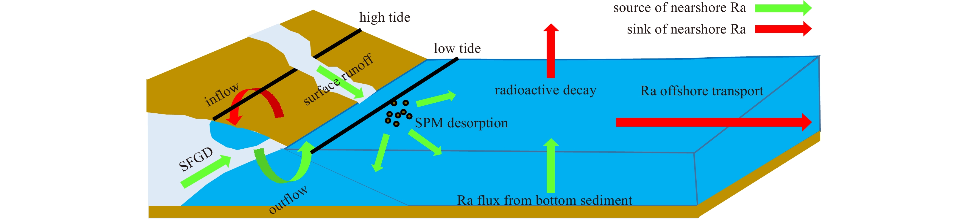
Figures(15) / Tables(8)

Supported by:
Beijing Renhe Information Technology Co. Ltd

Linwei Li, Jinzhou Du, Xilong Wang, Yanling Lao. Distinguishing the main components of submarine groundwater and estimating the corresponding fluxes based on radium tracing method—taking the Maowei Sea for example[J]. Acta Oceanologica Sinica, 2023, 42(8): 1-23. doi: 10.1007/s13131-023-2211-9

| Sample type | Parameter | Sampling date | |||
| June 2016 | March 2017 | January 2019 | May 2019 | ||
| GW AVG | Salinity | 0.2 | 0.2 | 0.2 | 0.2 |
| 224Ra activity concentration/(Bq·m−3) | 35.0 ± 1.6 | 23.6 ± 1.3 | 15.8 ± 1.8 | 8.0 ± 0.8 | |
| PW AVG | Salinity | 15.5 | 19.0 | 23.0 | 26.4 |
| 224Ra activity concentration/(Bq·m−3) | 486.5 ± 16.2 | 299.4 ± 9.0 | 484.4 ± 32.5 | 279.3 ± 14.0 | |
| RIV AVG | Salinity | 0.2 | 0.3 | 2.2 | 1.1 |
| 224Ra activity concentration/(Bq·m−3) | 3.1 ± 0.3 | 3.6 ± 0.3 | 11.2 ± 0.3 | 11.3 ± 1.0 | |
| PW EM | Salinity | 20.1 | 23.4 | 23.0 | 26.4 |
| 224Ra activity concentration/(Bq·m−3) | 486.5 ± 16.2 | 498.0 ± 10.6 | 484.4 ± 32.5 | 279.3 ± 14.0 | |
| Note: AVG means the average value; EM means the end member. | |||||
DownLoad:
CSV
| Parameter | Sampling date | ||||
| June 2016 | March 2017 | January 2019 | May 2019 | ||
| Salinity | Range | 2.5–12.6 | 19.3–25.6 | 13.7–27.9 | 6.6–18.9 |
| AVG | 7.3 | 21.8 | 21.6 | 12.8 | |
| 224Ra/(Bq·m−3) | Range | 7.9–33.0 | 9.9–31.6 | 4.8–13.4 | 5.3–20.2 |
| AVG | 12.8 | 18.3 | 9.1 | 16.1 | |
| Note: AVG means the average value. | |||||
DownLoad:
CSV
| Parameter | Value | Data source | Note |
| Ht/m | 2.4 | Zhang (2010) | tidal range |
| Tt/h | 24 | Zhang (2010) | tidal cycle |
| Hw/m | 0.52 | Zhang (2010) | wind wave height |
| Tw/s | 6 | Codification Committee of Gulf Records of China (1993) | wind wave period |
| h/m | 2.5 | Chen (2019) | mean water depth |
| g/(m2·s–1) | 9.8 | − | acceleration of Gravity |
| n | 0.4 | Wu (2012) | porosity |
| $\rho $/(g·cm−3) | 1.65 | Luo (2018) | sediment density |
| Salinity | 7.3 | field data | salinity |
| Kd/(cm3·g−1) | 840/S | Gu (2015) | solid-liquid partition coefficient |
| w/(m·s−1) | 5.4×10⁻¹¹ | Li et al. (2001) | deposition rate of suspended particulate matter |
| Dm0/(m2·s–1) | 8.0×10⁻¹⁰ | Li and Gregory (1974) | molecular diffusivity |
| $ \text{λ}$/s−1 | 2.17×10⁻⁶ | – | decay constant of 224Ra |
| $p$v | 0.04 | Appendix A | effective ejection volume ratio |
| ATh/(Bq·g−1) | 0.062 | Luo (2018) | activity of 228Th per unit mass of sediment |
DownLoad:
CSV
| Parameter | Position | Sampling time | |||
| June 2016 | March 2017 | January 2019 | May 2019 | ||
| Salinity | – | 7.3 | 21.8 | 20.4 | 12.8 |
| Kd/(cm3·g–1) | – | 115.1 | 38.5 | 41.2 | 65.6 |
| Csw/(m–3) | – | 7.9×10⁶ | 1.1×10⁷ | 4.7×10⁶ | 8.8×10⁶ |
| Kz/(m·s−1) | west | 1.4×10⁻³ | 1.8×10⁻³ | 1.2×10⁻³ | 2.9×10⁻³ |
| center | 1.4×10⁻³ | 2.8×10⁻³ | 9.0×10⁻⁴ | 3.0×10⁻³ | |
| east | 1.5×10⁻³ | 2.2×10⁻³ | 9.0×10⁻⁴ | 3.0×10⁻³ | |
| Dt0/(m2·s−1) | west | 8.4×10⁻¹² | 1.4×10⁻¹¹ | 6.2×10⁻¹² | 3.6×10⁻¹¹ |
| center | 8.4×10⁻¹² | 3.4×10⁻¹¹ | 3.5×10⁻¹² | 3.9×10⁻¹¹ | |
| east | 9.6×10⁻¹² | 2.1×10⁻¹² | 3.5×10⁻¹² | 3.9×10⁻¹¹ | |
| Dw0/(m2·s−1) | west | 4.7×10⁻⁹ | 7.7×10⁻⁹ | 3.4×10⁻⁹ | 2.0×10⁻⁸ |
| center | 4.7×10⁻⁹ | 1.9×10⁻⁸ | 1.9×10⁻⁹ | 2.1×10⁻⁸ | |
| east | 5.3×10⁻⁹ | 1.2×10⁻⁸ | 1.9×10⁻⁹ | 2.1×10⁻⁸ | |
| QB/(Bq·m−2·d−1) | west | 2.8 | 3.6 | 2.5 | 5.8 |
| center | 2.8 | 5.1 | 1.9 | 6.0 | |
| east | 3.0 | 4.3 | 1.9 | 6.0 | |
| QB_st/(Bq·m−2·d−1) | west | 2.6 | 3.5 | 2.3 | 5.7 |
| center | 2.6 | 5.0 | 1.6 | 5.9 | |
| east | 2.8 | 4.1 | 1.6 | 5.9 | |
| Fst/(m3·m–1·d−1) | west | 6.3×10³ | 1.7×10⁴ | 7.4×10³ | 3.1×10⁴ |
| center | 6.3×10³ | 2.0×10⁴ | 4.2×10³ | 2.9×10⁴ | |
| east | 7.2×10³ | 1.2×10⁴ | 4.2×10³ | 2.9×10⁴ | |
| Note: Kd is solid-liquid partition coefficient; Csw is 224Ra atom quantity concentration; Kz is vertical hydraulic conductivity of seafloor sediments; Dt0 is turbulent diffusion caused by tides; Dw0 is turbulent diffusion caused by wind waves; QB is Ra flux released from bottom sediments to overlying water; QB_st is the component of QB derived by tides and waves; Fst is the single-wide flux of submarine fresh groundwater discharge. | |||||
DownLoad:
CSV
| Parameter | Position | Sampling time | |||
| June 2016 | March 2017 | January 2019 | May 2019 | ||
| AC_f/(Bq·m−3) | − | 35.0 | 23.6 | 15.5 | 11.2 |
| AC_pw/(Bq·m−3) | – | 524.4 | 498.0 | 484.4 | 279.4 |
| AC_riv/(Bq·m−3) | – | 3.1 | 3.6 | 11.2 | 12.3 |
| *AC_0/(Bq·m–3) | west | 63.2 | 64.5 | 17.1 | 21.8 |
| center | 50.0 | 74.6 | 27.0 | 22.2 | |
| east | 40.4 | 75.7 | 21.1 | 21.9 | |
| AC_SPM/(Bq·g−1) | – | 0.062 | 0.062 | 0.062 | 0.062 |
| CSPM/(g·m−3) | – | 22.4 | 14.6 | 14.6 | 22.4 |
| $\eta $ | – | 0.3 | 0.3 | 0.3 | 0.3 |
| h/m | – | 2.5 | 2.5 | 2.5 | 2.5 |
| L/m | – | 1.3×10⁴ | 1.3×10⁴ | 1.3×10⁴ | 1.3×10⁴ |
| $\text{λ} $/s–1 | – | 2.17×10⁻⁶ | 2.17×10⁻⁶ | 2.17×10⁻⁶ | 2.17×10⁻⁶ |
| (P–E)/(mm·d−1) | – | 5.5 | −1.1 | −1.6 | 2.6 |
| Friv/(m3·m–1·d−1) | – | 172.8 | 29.3 | 21.1 | 111.4 |
| *u/(m·s−1) | west | 5.9×10⁻³ | 1.0×10⁻³ | 6.1×10⁻⁴ | 3.5×10⁻³ |
| center | 5.8×10⁻³ | 1.0×10⁻³ | 5.8×10⁻⁴ | 3.5×10⁻³ | |
| east | 5.9×10⁻³ | 1.0×10⁻³ | 6.5×10⁻⁴ | 3.5×10⁻³ | |
| *DL/(m·s−2) | west | 10.2 | 57.6 | 96.8 | 1073.0 |
| center | 10.0 | 42.1 | 28.5 | 720.8 | |
| east | 10.4 | 37.8 | 52.5 | 834.5 | |
| Note: AC_f is the 224Ra activity concentration of fresh groundwater end member; AC_pw is the 224Ra activity concentration of porewater end member; AC_riv is the 224Ra activity concentration of river water; *AC_0 is the 224Ra activity concentration of water in the land-sea boundary; AC_SPM is the 228Th activity of per unit mass sediment; CSPM is the mass concentration of suspended particulate matter in seawater; r in seawater; $\eta $ is maximum desorption ratio of Ra on the suspended particulate matter; h is the mean water depth; L is the spatial scale of the study water area; $ \text{λ} $ is the decay constant of 224Ra; P and E represent precipitation and evaporation in the study area, respectively; Friv is the surface runoff; *u is mean offshore velocity; *DL is turbulent diffusion coefficient of coastal water. The parameters labeled with * were obtained by fitting Eq. (17) with experimental data. AVG: average value. | |||||
DownLoad:
CSV
| Items | Position | Sampling time | |||
| June 2016 | March 2017 | January 2019 | May 2019 | ||
| Ff/(m3·m−1·d−1) | west | 132.2 | 115.6 | 62.4 | 85.5 |
| center | 211.4 | 35.0 | 36.1 | 95.7 | |
| east | 146.4 | 116.3 | 89.0 | 107.8 | |
| AVG | 163.3 | 89.0 | 62.5 | 163.3 | |
| Ftf/(m3·m−1·d−1) | west | 580.8 | 445.6 | 80.1 | 321.0 |
| center | 401.6 | 367.7 | 94.4 | 279.0 | |
| east | 307.9 | 351.7 | 79.7 | 254.6 | |
| AVG | 430.0 | 388.3 | 84.7 | 430.0 | |
| Note: Ff is the single-wide flux of SFGD; Ftf is the single-wide exchange capacity of tidal flat RSGD. AVG: average value. | |||||
DownLoad:
CSV
| Parameter | Value | |||||
| h/m | 2.5 | |||||
| L/m | 13000 | |||||
| DL/(m2·s−1) | 100 | |||||
| QB/(Bq·m–2·d−1) | 3 | |||||
| AC_0/(Bq·m−3) | 30 | |||||
| AC_f/(Bq·m−3) | 50 | |||||
| AC_pw/(Bq·m−3) | 500 | |||||
| AC_riv/(Bq·m−3) | 10 | |||||
| AC_SPM/(Bq·m−3) | 0.062 | |||||
| CSPM/(g·m−3) | 25 | |||||
| $\eta $ | 0.3 | |||||
| Kr0/m | 1×10⁵ | |||||
| Fr0/(m3·m−1·d−1) | 100 | |||||
| Kf0/m | 5×10³ | 1×10⁴ | 3×10⁴ | 7×10⁴ | 1×10⁵ | 1.2×10⁵ |
| Ff0/(m3·m–1·d–1) | 5 | 10 | 30 | 70 | 100 | 120 |
| Note: h is the mean water depth; L is the spatial scale of the study water area; DL is turbulent diffusion coefficient of coastal water. QB is Ra flux released from bottom sediments to overlying water; AC_0 is the 224Ra activity concentration of water in the land-sea boundary; AC_f is the 224Ra activity concentration of fresh groundwater endmember; AC_pw is the 224Ra activity concentration of porewater endmember; AC_riv is the 224Ra activity concentration of river water; AC_SPM is the 228Th activity of per unit mass suspended particulate matter; CSPM is the mass concentration of suspended particulate matter in seawater; $ \eta$ is maximum desorption ratio of Ra on the suspended particulate matter; Kr0 and Kf0 represent the increment of surface runoff or tidal flat submarine fresh groundwater discharge (SFGD) flux caused by an increase of one unit of net precipitation respectively; Fr0 and Ff0 represent the surface runoff or SFGD flux when the net precipitation is zero. | ||||||
DownLoad:
CSV
| Study area | Method or tracer | Date | Distance offshore from the low tide mark/m | Result | Reference | ||
| SGD | SFGD | RSGD | |||||
| Flamengo Bay near the city of Ubatuba, Sao Paulo State | seepage meter | Nov. 2003 | 10 | 2.6 m/d | 0.14 m/d | − | Taniguchi et al. (2008b) |
| 40 | 0.038 m/d | 2×10⁻³ m/d | − | Taniguchi et al. (2008b) | |||
| 50 | 1.86 m/d | 0.46 m/d | − | Taniguchi et al. (2008b) | |||
| Huanghe River Delta | seepage meter | Sept. 2004 | − | 8.04×10⁸ m3/d | 9.50×10⁶ m3/d | − | Taniguchi et al. (2008a) |
| May 2005 | − | 1.04×10⁸ m3/d | − | − | Taniguchi et al. (2008a) | ||
| Sept. 2006 | − | 1.73×10⁸ m3/d | 1.47×10⁷ m3/d | − | Taniguchi et al. (2008a) | ||
| North Liaodong Bay, Bohai Sea, China | Ra, water and salt balance model | Apr. and May 2017 | − | 1.48×10⁸−5.96× 10⁸ m3/d | 5.79×10⁷−6.66× 10⁷ m3/d | − | Zhang (2018) |
| Yellow Sea | 226Ra and 228Ra | Apr. and May 2014 | − | 2.14×10⁹−8.49× 10⁹ m3/d | 1.64×10⁷−11.2× 10⁷ m3/d | − | Liu et al. (2021) |
| Laizhou Bay, Bohai Sea | hydrological model | Sept. 2012 | − | − | 0.26 m3/(m·d) | 4.95 m3/(m·d)a, 1×10⁴ m3/(m·d)b | this study |
| Maowei Sea, Guangxi, China | 224Ra | Jun. 2016 | − | − | 163.33 m3/(m·d) | 430.09 m3/(m·d)a, 6.59×10³ m3/(m·d)b | this study |
| Mar. 2017 | − | − | 88.97 | 388.32 m3/(m·d)a, 1.64×10⁴ m3/(m·d)b | this study | ||
| Jan. 2019 | − | − | 62.48 | 84.73 m3/(m·d)a, 5.23×10³ m3/(m·d)b | this study | ||
| May 2015 | − | − | 163.33 | 430.09 m3/(m·d)a, 2.95×10⁴ m3/(m·d)b | this study | ||
| Note: SGD: submarine groundwater discharge; SFGD: submarine fresh groundwater discharge; RSGD: recirculated saline groundwater discharge; superscript a represents tidal flat RSGD; superscript b represents subtidal RSGD. − represents no data. | |||||||
DownLoad:
CSV
| Sample type | Parameter | Sampling date | |||
| June 2016 | March 2017 | January 2019 | May 2019 | ||
| GW AVG | Salinity | 0.2 | 0.2 | 0.2 | 0.2 |
| 224Ra activity concentration/(Bq·m−3) | 35.0 ± 1.6 | 23.6 ± 1.3 | 15.8 ± 1.8 | 8.0 ± 0.8 | |
| PW AVG | Salinity | 15.5 | 19.0 | 23.0 | 26.4 |
| 224Ra activity concentration/(Bq·m−3) | 486.5 ± 16.2 | 299.4 ± 9.0 | 484.4 ± 32.5 | 279.3 ± 14.0 | |
| RIV AVG | Salinity | 0.2 | 0.3 | 2.2 | 1.1 |
| 224Ra activity concentration/(Bq·m−3) | 3.1 ± 0.3 | 3.6 ± 0.3 | 11.2 ± 0.3 | 11.3 ± 1.0 | |
| PW EM | Salinity | 20.1 | 23.4 | 23.0 | 26.4 |
| 224Ra activity concentration/(Bq·m−3) | 486.5 ± 16.2 | 498.0 ± 10.6 | 484.4 ± 32.5 | 279.3 ± 14.0 | |
| Note: AVG means the average value; EM means the end member. | |||||
| Parameter | Sampling date | ||||
| June 2016 | March 2017 | January 2019 | May 2019 | ||
| Salinity | Range | 2.5–12.6 | 19.3–25.6 | 13.7–27.9 | 6.6–18.9 |
| AVG | 7.3 | 21.8 | 21.6 | 12.8 | |
| 224Ra/(Bq·m−3) | Range | 7.9–33.0 | 9.9–31.6 | 4.8–13.4 | 5.3–20.2 |
| AVG | 12.8 | 18.3 | 9.1 | 16.1 | |
| Note: AVG means the average value. | |||||
| Parameter | Value | Data source | Note |
| Ht/m | 2.4 | Zhang (2010) | tidal range |
| Tt/h | 24 | Zhang (2010) | tidal cycle |
| Hw/m | 0.52 | Zhang (2010) | wind wave height |
| Tw/s | 6 | Codification Committee of Gulf Records of China (1993) | wind wave period |
| h/m | 2.5 | Chen (2019) | mean water depth |
| g/(m2·s–1) | 9.8 | − | acceleration of Gravity |
| n | 0.4 | Wu (2012) | porosity |
| $\rho $/(g·cm−3) | 1.65 | Luo (2018) | sediment density |
| Salinity | 7.3 | field data | salinity |
| Kd/(cm3·g−1) | 840/S | Gu (2015) | solid-liquid partition coefficient |
| w/(m·s−1) | 5.4×10⁻¹¹ | Li et al. (2001) | deposition rate of suspended particulate matter |
| Dm0/(m2·s–1) | 8.0×10⁻¹⁰ | Li and Gregory (1974) | molecular diffusivity |
| $ \text{λ}$/s−1 | 2.17×10⁻⁶ | – | decay constant of 224Ra |
| $p$v | 0.04 | Appendix A | effective ejection volume ratio |
| ATh/(Bq·g−1) | 0.062 | Luo (2018) | activity of 228Th per unit mass of sediment |
| Parameter | Position | Sampling time | |||
| June 2016 | March 2017 | January 2019 | May 2019 | ||
| Salinity | – | 7.3 | 21.8 | 20.4 | 12.8 |
| Kd/(cm3·g–1) | – | 115.1 | 38.5 | 41.2 | 65.6 |
| Csw/(m–3) | – | 7.9×10⁶ | 1.1×10⁷ | 4.7×10⁶ | 8.8×10⁶ |
| Kz/(m·s−1) | west | 1.4×10⁻³ | 1.8×10⁻³ | 1.2×10⁻³ | 2.9×10⁻³ |
| center | 1.4×10⁻³ | 2.8×10⁻³ | 9.0×10⁻⁴ | 3.0×10⁻³ | |
| east | 1.5×10⁻³ | 2.2×10⁻³ | 9.0×10⁻⁴ | 3.0×10⁻³ | |
| Dt0/(m2·s−1) | west | 8.4×10⁻¹² | 1.4×10⁻¹¹ | 6.2×10⁻¹² | 3.6×10⁻¹¹ |
| center | 8.4×10⁻¹² | 3.4×10⁻¹¹ | 3.5×10⁻¹² | 3.9×10⁻¹¹ | |
| east | 9.6×10⁻¹² | 2.1×10⁻¹² | 3.5×10⁻¹² | 3.9×10⁻¹¹ | |
| Dw0/(m2·s−1) | west | 4.7×10⁻⁹ | 7.7×10⁻⁹ | 3.4×10⁻⁹ | 2.0×10⁻⁸ |
| center | 4.7×10⁻⁹ | 1.9×10⁻⁸ | 1.9×10⁻⁹ | 2.1×10⁻⁸ | |
| east | 5.3×10⁻⁹ | 1.2×10⁻⁸ | 1.9×10⁻⁹ | 2.1×10⁻⁸ | |
| QB/(Bq·m−2·d−1) | west | 2.8 | 3.6 | 2.5 | 5.8 |
| center | 2.8 | 5.1 | 1.9 | 6.0 | |
| east | 3.0 | 4.3 | 1.9 | 6.0 | |
| QB_st/(Bq·m−2·d−1) | west | 2.6 | 3.5 | 2.3 | 5.7 |
| center | 2.6 | 5.0 | 1.6 | 5.9 | |
| east | 2.8 | 4.1 | 1.6 | 5.9 | |
| Fst/(m3·m–1·d−1) | west | 6.3×10³ | 1.7×10⁴ | 7.4×10³ | 3.1×10⁴ |
| center | 6.3×10³ | 2.0×10⁴ | 4.2×10³ | 2.9×10⁴ | |
| east | 7.2×10³ | 1.2×10⁴ | 4.2×10³ | 2.9×10⁴ | |
| Note: Kd is solid-liquid partition coefficient; Csw is 224Ra atom quantity concentration; Kz is vertical hydraulic conductivity of seafloor sediments; Dt0 is turbulent diffusion caused by tides; Dw0 is turbulent diffusion caused by wind waves; QB is Ra flux released from bottom sediments to overlying water; QB_st is the component of QB derived by tides and waves; Fst is the single-wide flux of submarine fresh groundwater discharge. | |||||
| Parameter | Position | Sampling time | |||
| June 2016 | March 2017 | January 2019 | May 2019 | ||
| AC_f/(Bq·m−3) | − | 35.0 | 23.6 | 15.5 | 11.2 |
| AC_pw/(Bq·m−3) | – | 524.4 | 498.0 | 484.4 | 279.4 |
| AC_riv/(Bq·m−3) | – | 3.1 | 3.6 | 11.2 | 12.3 |
| *AC_0/(Bq·m–3) | west | 63.2 | 64.5 | 17.1 | 21.8 |
| center | 50.0 | 74.6 | 27.0 | 22.2 | |
| east | 40.4 | 75.7 | 21.1 | 21.9 | |
| AC_SPM/(Bq·g−1) | – | 0.062 | 0.062 | 0.062 | 0.062 |
| CSPM/(g·m−3) | – | 22.4 | 14.6 | 14.6 | 22.4 |
| $\eta $ | – | 0.3 | 0.3 | 0.3 | 0.3 |
| h/m | – | 2.5 | 2.5 | 2.5 | 2.5 |
| L/m | – | 1.3×10⁴ | 1.3×10⁴ | 1.3×10⁴ | 1.3×10⁴ |
| $\text{λ} $/s–1 | – | 2.17×10⁻⁶ | 2.17×10⁻⁶ | 2.17×10⁻⁶ | 2.17×10⁻⁶ |
| (P–E)/(mm·d−1) | – | 5.5 | −1.1 | −1.6 | 2.6 |
| Friv/(m3·m–1·d−1) | – | 172.8 | 29.3 | 21.1 | 111.4 |
| *u/(m·s−1) | west | 5.9×10⁻³ | 1.0×10⁻³ | 6.1×10⁻⁴ | 3.5×10⁻³ |
| center | 5.8×10⁻³ | 1.0×10⁻³ | 5.8×10⁻⁴ | 3.5×10⁻³ | |
| east | 5.9×10⁻³ | 1.0×10⁻³ | 6.5×10⁻⁴ | 3.5×10⁻³ | |
| *DL/(m·s−2) | west | 10.2 | 57.6 | 96.8 | 1073.0 |
| center | 10.0 | 42.1 | 28.5 | 720.8 | |
| east | 10.4 | 37.8 | 52.5 | 834.5 | |
| Note: AC_f is the 224Ra activity concentration of fresh groundwater end member; AC_pw is the 224Ra activity concentration of porewater end member; AC_riv is the 224Ra activity concentration of river water; *AC_0 is the 224Ra activity concentration of water in the land-sea boundary; AC_SPM is the 228Th activity of per unit mass sediment; CSPM is the mass concentration of suspended particulate matter in seawater; r in seawater; $\eta $ is maximum desorption ratio of Ra on the suspended particulate matter; h is the mean water depth; L is the spatial scale of the study water area; $ \text{λ} $ is the decay constant of 224Ra; P and E represent precipitation and evaporation in the study area, respectively; Friv is the surface runoff; *u is mean offshore velocity; *DL is turbulent diffusion coefficient of coastal water. The parameters labeled with * were obtained by fitting Eq. (17) with experimental data. AVG: average value. | |||||
| Items | Position | Sampling time | |||
| June 2016 | March 2017 | January 2019 | May 2019 | ||
| Ff/(m3·m−1·d−1) | west | 132.2 | 115.6 | 62.4 | 85.5 |
| center | 211.4 | 35.0 | 36.1 | 95.7 | |
| east | 146.4 | 116.3 | 89.0 | 107.8 | |
| AVG | 163.3 | 89.0 | 62.5 | 163.3 | |
| Ftf/(m3·m−1·d−1) | west | 580.8 | 445.6 | 80.1 | 321.0 |
| center | 401.6 | 367.7 | 94.4 | 279.0 | |
| east | 307.9 | 351.7 | 79.7 | 254.6 | |
| AVG | 430.0 | 388.3 | 84.7 | 430.0 | |
| Note: Ff is the single-wide flux of SFGD; Ftf is the single-wide exchange capacity of tidal flat RSGD. AVG: average value. | |||||
| Parameter | Value | |||||
| h/m | 2.5 | |||||
| L/m | 13000 | |||||
| DL/(m2·s−1) | 100 | |||||
| QB/(Bq·m–2·d−1) | 3 | |||||
| AC_0/(Bq·m−3) | 30 | |||||
| AC_f/(Bq·m−3) | 50 | |||||
| AC_pw/(Bq·m−3) | 500 | |||||
| AC_riv/(Bq·m−3) | 10 | |||||
| AC_SPM/(Bq·m−3) | 0.062 | |||||
| CSPM/(g·m−3) | 25 | |||||
| $\eta $ | 0.3 | |||||
| Kr0/m | 1×10⁵ | |||||
| Fr0/(m3·m−1·d−1) | 100 | |||||
| Kf0/m | 5×10³ | 1×10⁴ | 3×10⁴ | 7×10⁴ | 1×10⁵ | 1.2×10⁵ |
| Ff0/(m3·m–1·d–1) | 5 | 10 | 30 | 70 | 100 | 120 |
| Note: h is the mean water depth; L is the spatial scale of the study water area; DL is turbulent diffusion coefficient of coastal water. QB is Ra flux released from bottom sediments to overlying water; AC_0 is the 224Ra activity concentration of water in the land-sea boundary; AC_f is the 224Ra activity concentration of fresh groundwater endmember; AC_pw is the 224Ra activity concentration of porewater endmember; AC_riv is the 224Ra activity concentration of river water; AC_SPM is the 228Th activity of per unit mass suspended particulate matter; CSPM is the mass concentration of suspended particulate matter in seawater; $ \eta$ is maximum desorption ratio of Ra on the suspended particulate matter; Kr0 and Kf0 represent the increment of surface runoff or tidal flat submarine fresh groundwater discharge (SFGD) flux caused by an increase of one unit of net precipitation respectively; Fr0 and Ff0 represent the surface runoff or SFGD flux when the net precipitation is zero. | ||||||
| Study area | Method or tracer | Date | Distance offshore from the low tide mark/m | Result | Reference | ||
| SGD | SFGD | RSGD | |||||
| Flamengo Bay near the city of Ubatuba, Sao Paulo State | seepage meter | Nov. 2003 | 10 | 2.6 m/d | 0.14 m/d | − | Taniguchi et al. (2008b) |
| 40 | 0.038 m/d | 2×10⁻³ m/d | − | Taniguchi et al. (2008b) | |||
| 50 | 1.86 m/d | 0.46 m/d | − | Taniguchi et al. (2008b) | |||
| Huanghe River Delta | seepage meter | Sept. 2004 | − | 8.04×10⁸ m3/d | 9.50×10⁶ m3/d | − | Taniguchi et al. (2008a) |
| May 2005 | − | 1.04×10⁸ m3/d | − | − | Taniguchi et al. (2008a) | ||
| Sept. 2006 | − | 1.73×10⁸ m3/d | 1.47×10⁷ m3/d | − | Taniguchi et al. (2008a) | ||
| North Liaodong Bay, Bohai Sea, China | Ra, water and salt balance model | Apr. and May 2017 | − | 1.48×10⁸−5.96× 10⁸ m3/d | 5.79×10⁷−6.66× 10⁷ m3/d | − | Zhang (2018) |
| Yellow Sea | 226Ra and 228Ra | Apr. and May 2014 | − | 2.14×10⁹−8.49× 10⁹ m3/d | 1.64×10⁷−11.2× 10⁷ m3/d | − | Liu et al. (2021) |
| Laizhou Bay, Bohai Sea | hydrological model | Sept. 2012 | − | − | 0.26 m3/(m·d) | 4.95 m3/(m·d)a, 1×10⁴ m3/(m·d)b | this study |
| Maowei Sea, Guangxi, China | 224Ra | Jun. 2016 | − | − | 163.33 m3/(m·d) | 430.09 m3/(m·d)a, 6.59×10³ m3/(m·d)b | this study |
| Mar. 2017 | − | − | 88.97 | 388.32 m3/(m·d)a, 1.64×10⁴ m3/(m·d)b | this study | ||
| Jan. 2019 | − | − | 62.48 | 84.73 m3/(m·d)a, 5.23×10³ m3/(m·d)b | this study | ||
| May 2015 | − | − | 163.33 | 430.09 m3/(m·d)a, 2.95×10⁴ m3/(m·d)b | this study | ||
| Note: SGD: submarine groundwater discharge; SFGD: submarine fresh groundwater discharge; RSGD: recirculated saline groundwater discharge; superscript a represents tidal flat RSGD; superscript b represents subtidal RSGD. − represents no data. | |||||||
 DownLoad: