Weizhen Jiang, Guizhi Wang, Qing Li, Manab Kumar Dutta, Shilei Jin, Guiyuan Dai, Yi Xu. The fate of carbon resulting from pore water exchange in a mangrove and Spartina alterniflora ecozone[J]. Acta Oceanologica Sinica, 2023, 42(8): 61-76. doi: 10.1007/s13131-023-2234-2
Citation:
Weizhen Jiang, Guizhi Wang, Qing Li, Manab Kumar Dutta, Shilei Jin, Guiyuan Dai, Yi Xu. The fate of carbon resulting from pore water exchange in a mangrove and Spartina alterniflora ecozone[J]. Acta Oceanologica Sinica, 2023, 42(8): 61-76. doi: 10.1007/s13131-023-2234-2
Weizhen Jiang, Guizhi Wang, Qing Li, Manab Kumar Dutta, Shilei Jin, Guiyuan Dai, Yi Xu. The fate of carbon resulting from pore water exchange in a mangrove and Spartina alterniflora ecozone[J]. Acta Oceanologica Sinica, 2023, 42(8): 61-76. doi: 10.1007/s13131-023-2234-2
Citation:
Weizhen Jiang, Guizhi Wang, Qing Li, Manab Kumar Dutta, Shilei Jin, Guiyuan Dai, Yi Xu. The fate of carbon resulting from pore water exchange in a mangrove and Spartina alterniflora ecozone[J]. Acta Oceanologica Sinica, 2023, 42(8): 61-76. doi: 10.1007/s13131-023-2234-2
State Key Laboratory of Marine Environmental Science, Xiamen University, Xiamen 361102, China
2.
College of Ocean and Earth Sciences, Xiamen University, Xiamen 361102, China
3.
Fujian Provincial Key Laboratory for Coastal Ecology and Environmental Studies, Xiamen University, Xiamen 361102, China
4.
National Observation and Research Station for the Taiwan Strait Marine Ecosystem, Xiamen University, Zhangzhou 363000, China
5.
Key Laboratory of Coastal Environment and Resources of Zhejiang Province, School of Engineering, Westlake University, Hangzhou 310000, China
Funds:
The Fund of Ministry of Science and Technology of China under contract No. 2022YFC3105402; the Natural Science Foundation of Fujian Province of China under contract No. 2019J01020; the National Natural Science Foundation of China under contract No. 42141001; the Fujian Provincial Central Guided Local Science and Technology Development Special Project under contract No. 2022L3078.
Mangrove and salt-marsh wetlands are important coastal carbon sinks. In order to quantify carbon export via pore water exchange and to evaluate subsequent fate of the exported carbon, we carried out continuous observations in a mangrove-Spartina alterniflora ecozone in the Zhangjiang River Estuary, China. The carbon fluxes via pore water exchange were estimated using 222Rn and 228Ra as tracers to be (2.15 ± 0.63) mol/(m2∙d) for dissolved inorganic carbon (DIC) and (–0.008 ± 0.07) mol/(m2∙d) for dissolved organic carbon (DOC) in the wet season and (3.02 ± 0.65) mol/(m2∙d) for DIC and (–0.15 ± 0.007) mol/(m2∙d) for DOC in the dry season in the mangrove-dominated creek (M-creek), while (2.52 ± 0.82) mol/(m2∙d) for DIC and (0.02 ± 0.09) mol/(m2∙d) for DOC in the dry season in the S. alterniflora-dominated creek (SA-creek). The negative value means that pore water was a sink of DOC in the creek. The total carbon via pore water exchange in the tidal creeks in the mangroves accounted for 41%–55% of the net carbon fixed by mangrove vegetation and was 3–4 times as much as the soil carbon accretion in the mangroves. The exported carbon in the form of DIC contributed all of the carbon outwelling from the M-creek and 79% of the carbon outwelling from the SA-creek, implying effective fixation of carbon by the wetland ecosystem. Moreover, it resulted in 54% in the dry season, 75% in the wet season of the carbon dioxide released from the M-creek to the atmosphere, and 84% of the release from the SA-creek. Therefore, quantification of pore water exchange and related soil carbon loss is essential to trace the fate of carbon fixed in intertidal wetlands.
Mangroves are a remarkable blue carbon sink system on Earth with a global carbon storage of 4.19 Pg, of which 2.96 Pg is locked in the soil (Hamilton and Friess, 2018). They are among the forests with the highest carbon storage in the soil on the planet at the Millennium scale (Atwood et al., 2017; Choi and Wang, 2004; Donato et al., 2011; Maher et al., 2017). Although mangroves cover only 0.5% of the global coastal area, the carbon stored in the mangrove soils, 24 Tg/a, accounts for 10%–15% of the carbon preserved in coastal sediments (Alongi, 2014). Recent evidences further indicate that considerable amounts of the carbon, equivalent to 30%–40% of the global riverine organic carbon flux, that should have been buried in the soil have been lost (Hamilton and Friess, 2018; Bouillon et al., 2008). One invisible pathway of the soil carbon exported to the coastal water is via pore water exchange and/or submarine groundwater discharge with a potential loss rate 40% as high as the annual primary production of mangroves (Alongi, 2014). The transport efficiency of this pathway is affected by sediment properties such as particle size and permeability (Konikow et al., 2013; Robinson et al., 2007). Mangrove sediments are mostly silty clay up to 5–7 m deep with low permeability and strong viscosity, so the discharge of fresh groundwater is generally hindered (Whelan et al., 2005). In mangroves, therefore, pore water exchange is the main pathway of material exchange between the sediment and tidal creek water.
The pore water exchange in mangroves has been described as a mangrove pump (Tait et al., 2016). At high tides, the water from tidal creeks enters the pores densely distributed in the soils due to pressure gradients, and flows out at low tides, carrying large amounts of dissolved substances, such as dissolved inorganic carbon (DIC), dissolved organic carbon (DOC), and nutrients, into the tidal creeks (Maher et al., 2013; Santos et al., 2019; Reithmaier et al., 2021). Recent studies have shown that about 5.6 Tg of soil carbon in global mangrove systems has been laterally exported into nearshore waters every year, 75%–80% of which is discharged in the form of DIC (Alongi, 2014, 2020; Chen et al., 2018; Ray et al., 2018), which explains why mangrove tidal creeks are shown to be a main source of atmospheric CO2 (Santos et al., 2012; Chen et al., 2021b).
Invasion of S. alterniflora along the Chinese coast has become a widespread environmental concern from the Bohai Sea southward to Hainan Island over the past few decades (Chen, 2021). For example, in the Zhangjiang River Estuary, the areal extent of S. alterniflora in the native mangrove system had doubled during 2003–2015 (Liu et al., 2017), thus forming an ecotone of mangrove-S. alterniflora. Previous studies have advanced our understanding of the impact of pore water input in mangrove tidal creeks on the carbon cycle (Kristensen et al., 2008; Call et al., 2019), but pore water exchange and related carbon cycle still remain relatively understudied on ecotone formed under the invasion of S. alterniflora. Does the carbon flux via pore water exchange in the Spartina-dominated area differ from the mangrove-dominated area? What is the subsequent fate of the dissolved carbon exported from the soil to the creeks via pore water exchange in both areas?
In order to explore the fate of carbon exported via pore water exchange and to compare the mangrove-dominated system with the Spartina-dominated system, we have utilized radium and radon as pore water tracers to calculate the DIC and DOC fluxes via pore water exchange in the subtropical mangrove-S. alterniflora ecotone in the Zhangjiang River Estuary.
2.
Materials and methods
2.1
Study area
The Zhangjiang River Estuary Mangrove National Nature Reserve is located in the subtropical Zhangjiang River Estuary in Fujian Province, China (23.91°−23.93°N, 117.41°−117.43°E) (Fig. 1). The whole terrain descends from northwest to southeast, forming a horseshoe-shaped landform opening to the southeast. Many creeks are distributed in the mangrove forest, and finally converge with the main stream of the Zhangjiang River before flowing into the Dongshan Bay and further into the Taiwan Strait (Zhang et al., 2013). This area is influenced by the East Asian monsoons, with annual average temperature of 21.2℃, wind speed of 2.7 m/h, and precipitation of 1 715 mm (Gao et al., 2018). The creeks are affected by irregular semi-diurnal tides with a range of 0.43–4.67 m and an average of 2.32 m (Chen et al., 2010b; Hui et al., 2006). Some coastal vegetations are submerged during flood tides, and large areas of mudflats are exposed at ebb tides (Chen et al., 2010b). The dominant species of mangroves in the Zhangjiang River Estuary are Kandeliaobovata, Aegiceras corniculatum, and Avicennia marina (Feng et al., 2017). The mangrove roots usually develop within 90 cm of the ground surface (Lin, 2019). They play an important role in preventing soil erosion and storing buried carbon in the soil. However, the mangrove soils are mainly composed of silty clay with thickness of more than 2 m (Li et al., 2018), so the roots of these mangroves cannot penetrate the low permeability soil layer so as for terrestrial groundwater in the deep aquifer to upwell. Exchanges between the soil and creek waters are mainly via densely distributed biological pores in the soil (Ridd, 1996).
Figure
1.
Study area and sampling stations. a. Location of the study site; b. the sampling stations; c. the stations in the tidal creeks; d. the mangrove-dominated area (Station TS1); e. the Spartina alterniflora-dominated area (Station TS2).
Field observations were conducted during September 2–4, 2018 (wet season) and March 9–11, 2019 (dry season) in the mangrove-Spartina ecotone of Zhangjiang River Estuary (Fig. 1b). Time-series observations were carried out in tidal creeks at Station TS1 (23.927 2°N, 117.417 2°E) in the mangrove-dominated area in both seasons and at Station TS2 (23.922 2°N, 117.423 1°E), which is at the edge of the mangrove forest with serious invasion of S. alterniflora and about 400 m away from Station TS1, in the dry season (Figs 1c-e). Unlike Station TS1 where the coast was covered by mangroves, Station TS2 had a coast of exposed mudflats where S. alterniflora invaded. Hydrographic parameters, temperature, water depth, and salinity were determined with Aqua TROLL 200 (In-Situ Inc., USA). The meteorological parameters, wind speed and air pressure were measured with an automatic weather station (R.M. YOUNG, USA). Water samples were taken for 222Rn, 226Ra, 228Ra, DIC, total alkalinity (TA) and DOC every 2 h for 24 h at the two stations using a glass water sampler. In addition, we sampled the Zhangjiang River water, seawater, pore water, and well water for the same parameters during the same period. Water samples from the Zhangjiang River, seawater, and domestic wells were collected in the same way as the tidal creek water. Pore water samples were collected during the ebb tide by digging bores to a depth of about 50 cm and waiting for the water to converge naturally at the edge of the tidal creek in the mangroves. The water in each bore was purged at least three times before sample collection. We used a WTW Multi 340i to measure the temperature and salinity of water samples after each collection. Unfortunately, at Station TS2 we failed to measure the partial pressure of carbon dioxide (pCO2) due to equipment failure. The pCO2 value was calculated using CO2SYS (Pelletier et al., 2015) using measured DIC, TA, salinity and temperature. As the weather station was damaged at Station TS2, the average values of wind speed and air pressure at Station TS1 on the same day were used. 222Rn samples were collected in 250 mL bottles and the activity of 222Rn was determined with RAD7 (Durridge Co., USA) using Water 250 protocol right after sampling. In addition, sediment cores were collected with 65 mm-diameter PVC pipes to estimate diffusive fluxes of 222Rn across the sediment-water interface using a sediment equilibration method detailed in Corbett et al. (1998). A Rhizon sampling system (the Netherlands) was used to collect pore water in the cores as detailed in Seeberg-Elverfeldt et al. (2005). We used PICARRO G2101-i and PICARRO G2132-i (USA) to measure pCO2in situ.
In the field, water samples for 226Ra and 228Ra were enriched for radium with 16 g of MnO2-coated fibers (Mn-fibers) at a flow rate of less than 0.6 L/min immediately after collection following the procedure in Moore and Arnold (1996). The Mn-fibers were washed with deionized water to remove the salt and particles. DIC and TA samples were collected in 250 mL borosilicate glass bottles and preserved with saturated HgCl2. For DOC, samples were collected in 40 mL dark glass bottles after filtration through a syringe filter assembled with a pre-burned (450℃ for 5 h) GF/F membrane, then preserved with H3PO4 before being kept at −20℃ until further analysis.
2.3
Laboratory analysis
The radium adsorbed on the Mn-fiber was leached with a mixture of 1 mol/L hydroxylamine hydrochloride and 1 mol/L HCl at a ratio of 2:1 at 80℃. Then, saturated Ba(NO3)2 and 1 mol/L NaHSO4 were added to the solution to co-precipitate radium with BaSO4. The precipitate was stored for 21 d before being measured with a germanium gamma detector (GCW4022, Canberra, Germany). The measurement error of 226Ra and 228Ra was less than 5%.
DIC and TA samples were equilibrated at 25℃ before measurements. The concentration of DIC was measured using a DIC analyser (Apollo, USA). The concentration of TA was determined using an automatic alkalinity titrator (Apollo, USA). Both determinations of DIC and TA were corrected with reference seawater (provided by Andrew Dickson, the Scripps Institution of Oceanography, USA), and the measurement errors were less than 0.1%.
For DOC, the refrigerated samples were first thawed at a laboratory temperature and then analyzed using a total organic carbon (TOC) analyzer (Shimadzu TOC-V CPH, Japan). Certified reference materials (from Hansell Laboratory at University of Miami) were used for DOC quality control.
2.4
Estimation of the pore water exchange rate using radioactive tracers
In this study, in order to ensure the reliability of our results, two radioactive tracers, 222Rn and 228Ra, were collected to estimate the pore water exchange rate for comparison. Similar to the 222Rn mass balance model established by Chen et al. (2018), we established a mass balance model of 228Ra for comparison.
2.4.1
The mass balance model of222Rn
The sources of 222Rn in the tidal creeks include the river, pore water exchange, sediment diffusion, and the ingrowth from 226Ra. The sinks are decay, atmospheric evasion, tidal effects, and mixing with the seawater. At each time-series station, the mass balance model of 222Rn is as follows (Chen et al., 2018):
where FR1 and FPW1 are the flux of 222Rn attributed by the river and pore water exchange; FS1 is diffusion flux from the sediment; and FRa is the ingrowth from 226Ra. Fin1 and Fout1 are the influx and outflux due to tides, respectively. FA is the atmospheric evasion flux; FD is the decay of radon; FM1 is the flux due to mixing with the seawater; and $ {\Delta F}_{1} $ is the difference of 222Rn inventory between two consecutive sampling time points. The unit is in Bq/(m2∙s). It and $ {I}_{t+\Delta t} $(Bq/m2) are the 222Rn inventory at time t and t+$ \Delta t $; t (s) is the sampling time, and $ \Delta t $ is the sampling interval.
The monthly average discharge of the Zhangjiang River in March and September of 2019 is 20.8 m3/s and 21.7 m3/s, respectively. FR1 can be obtained by the river discharge multiplied by the 222Rn concentration of the river endmember.
where h is the water depth, $ {\overline{C}}_{\mathrm{c}\mathrm{r}\mathrm{e}\mathrm{e}\mathrm{k}} $(Bq/m3) is the mean 222Rn concentration in the tidal creeks, $ {C}_{\mathrm{S}\mathrm{W}} $ (Bq/m3) is the 222Rn concentration of the seawater endmember, $ {C}_{\mathrm{c}\mathrm{r}\mathrm{e}\mathrm{e}\mathrm{k}} $ (Bq/m3) is the 222Rn concentration in the tidal creeks, and b is the return flow factor. Under the assumption that the Ra desorbed from suspended particles was negligible, which is verified later in Section 3.4, we used a three-endmember mixing model to estimate the fraction of seawater, which was taken as b (Moore et al., 2006):
where fR, fPW and fSW are the fraction of river water, pore water, and seawater endmembers; SR, SPW and SSW are the salinity of river water, pore water, and seawater endmembers; $ {{}_{}{}^{228}\mathrm{R}\mathrm{a}}_{\mathrm{R}} $, $ {{}_{}{}^{228}\mathrm{R}\mathrm{a}}_{\mathrm{P}\mathrm{W}} $ and $ {{}_{}{}^{228}\mathrm{R}\mathrm{a}}_{\mathrm{S}\mathrm{W}} $ are the activity concentrations of 228Ra of river water, pore water, and seawater endmembers. The subscript M refers to the measured value at the time series station.
The supported flux of 222Rn by 226Ra decay (FRa) and the decay of 222Rn (FD) are as follows:
where $ \phi $ is the porosity of sediments; Dm is the molecular diffusion coefficient of 222Rn; $ {C}_{\mathrm{e}\mathrm{q}} $ (Bq/m3) is the 222Rn concentration in the interstitial water of sediments; and T is the water temperature (℃).
where $ {k}_{1} $ is the transfer velocity of 222Rn; α is the partition coefficient; and $ {C}_{\mathrm{a}\mathrm{i}\mathrm{r}} $ (Bq/m3) is the 222Rn activity in air. α is defined by the Fritz Weigel equation (Burnett and Dulaiova, 2003):
where u is the wind speed, when u < 3.6 m/s, X = 0.666 7, and when u > 3.6 m/s, X = 0.5. $ {S}_{{\mathrm{C}}_{1}} $ is the Schmidt number of radon and the calculation method refers to Pilson (2013) and Wanninkhof (1992):
where ν is the kinematic viscosity (m2/s), A (in 10−9 m2/s) and E (the energy of activation of diffusion, J/mol) are fitting parameters, and R is the gas constant (8.314 5 J/(mol∙K)).
The mixing loss was estimated by the net 222Rn flux after corrections for tidal effect, 226Ra ingrowth, sediment diffusion, the decay of 222Rn, and atmospheric loss. The net 222Rn flux is described as follows (Zhang et al., 2016):
We chose the maximum negative Fnet as a conservative estimate of FM (mixing loss) as suggested by Burnett and Dulaiova (2003). Fnet should be a balance between FPW and FM. So, the 222Rn flux contributed by pore water is
We used the conservative estimate of FM to calculate the minimum FPW. The rate of pore water exchange (ω, cm/s) was obtained by FPW divided by the 222Rn concentration in the pore water endmember (CPW):
228Ra has no atmospheric evasion, but desorption from particles has to be taken into account. The half-life of 228Ra is 5.75 a, so that its decay can be ignored in a tidal cycle. Similar to 222Rn, a mass balance model of 228Ra was set up as following to estimate the rate of pore water exchange:
where FR2 and FPW2 are the flux of 228Ra attributed by the river and pore water exchange; Fin2 and Fout2 are the influx and outflux due to tides, respectively; FM2 is the flux due to mixing with the seawater; and $ {\Delta F}_{2} $ is the difference of 228Ra inventory between two consecutive sampling time points. FP is the desorption flux from suspended particles, which can be obtained by multiplying the river discharge by the particle concentration and then by the particle desorption coefficient of 228Ra. The unit is in dpm/(m2∙s) (1 Bq = 60 dpm). We used the maximum desorption coefficient, PRa-228 = 0.899 dpm/g, and FS2 of 2.1 dpm/(m2∙d) from Krest et al. (1999) in this calculation. The rate of pore water exchange was calculated similar to the 222Rn mass balance model.
2.5
Estimation of the flux of dissolved carbon via pore water exchange
The net carbon flux via pore water exchange into the tidal creeks was estimated using the average 222Rn-based advection rate multiplied by the difference between the concentrations of dissolved carbon in the pore water and in the tidal creeks.
2.6
Estimation of the air-water CO2flux
The flux of air-water CO2 ($ {F}_{\mathrm{C}{\mathrm{O}}_{2}} $) depends on difference between the pCO2 in water and the pCO2 in the atmosphere and environmental factors such as water temperature, salinity, and wind speed. The $ {F}_{{\mathrm{C}\mathrm{O}}_{2}} $ (Sweeney et al., 2007) was calculated as
where A and B are constants, the unit is in mol/(kg∙atm) (1 atm = 101 325 Pa). T is absolute temperature and S is salinity. A1 = −60.240 9, A2 = 93.451 7, A3 = 23.358 5, B1 = 0.023 517, B2 = −0.023 656 and B3 = 0.004 736.
$ \Delta p{\mathrm{C}\mathrm{O}}_{2} $ is the difference between the pCO2 in the creek water and in the atmosphere, and $ {k}_{2} $ is the gas transfer velocity of CO2 calculated as
where u is the wind speed, when u < 3.6 m/s, X = 0.666 7, and when u > 3.6 m/s, X = 0.5. $ {S}_{{\mathrm{C}}_{2}} $ is the Schmidt number of CO2 (Pilson, 2013; Wanninkhof, 1992).
2.7
Estimation of the CO2emission from the tidal creeks in the mangrove-Spartina ecozone contributed by pore water exchange
To determine the emission of CO2 from the creeks contributed by pore water exchange, we calculated the pCO2 resulting from pore water exchange in the creek based on the mass balance of DIC and TA in the creeks. Firstly, the concentration of DIC without the contribution of pore water exchange was designated as DIC0 and was estimated as follows. The DIC inventory in the creek was obtained by
$$ {I}_{\mathrm{C}}={C}_{\mathrm{C}}\times V , $$
(23)
where IC is the inventory of DIC in the creek; CC is the DIC concentration in the creek; and V is the volume of water in the creek. The inventory of DIC contributed by seawater (ISW) was calculated as
$$ {I}_{\mathrm{S}\mathrm{W}}=V\times {C}_{\mathrm{S}\mathrm{W}}\times b , $$
(24)
where CSW is the DIC concentration of the seawater endmember. Since the total DIC inventory in the study area was mainly contributed by seawater, pore water exchange, river water and sediments, the contribution of pore water exchange, river water and sediments to the total inventory can be obtained by subtracting the contribution of seawater from the total DIC inventory. The inventory of DIC contributed by pore water exchange (IPW) was thus calculated as
where FPW, FS, and FR denote the flux of DIC associated with pore water exchange, sediment, and the Zhangjiang River, respectively. The concentration of DIC without the contribution of pore water exchange (DIC0) was calculated as
Similarly, the concentration of TA without the contribution of pore water exchange (TA0) was obtained. Secondly, the pCO2 in the creek without pore water exchange contribution ($ p\mathrm{C}{\mathrm{O}}_{{2}_{0}} $) was calculated from DIC0 and TA0 with CO2SYS using in-situ temperature and salinity. Thirdly, the pCO2 resulting from pore water exchange in the creek was estimated by subtracting $ p\mathrm{C}{\mathrm{O}}_{{2}_{0}} $ from the measured pCO2 in the creek. The air-water CO2 flux without the influence of pore water exchange ($ {F}_{\mathrm{C}{\mathrm{O}}_{{2}_{0}}} $) was calculated using $ p\mathrm{C}{\mathrm{O}}_{{2}_{0}} $ and the atmospheric pCO2 with Eq. (20). The air-water CO2 flux contributed by pore water exchange ($ {F}_{\mathrm{C}{\mathrm{O}}_{{2}_{\mathrm{P}\mathrm{W}}}} $) was estimated as
3.1
Features of the pore water, well water, and river water endmembers
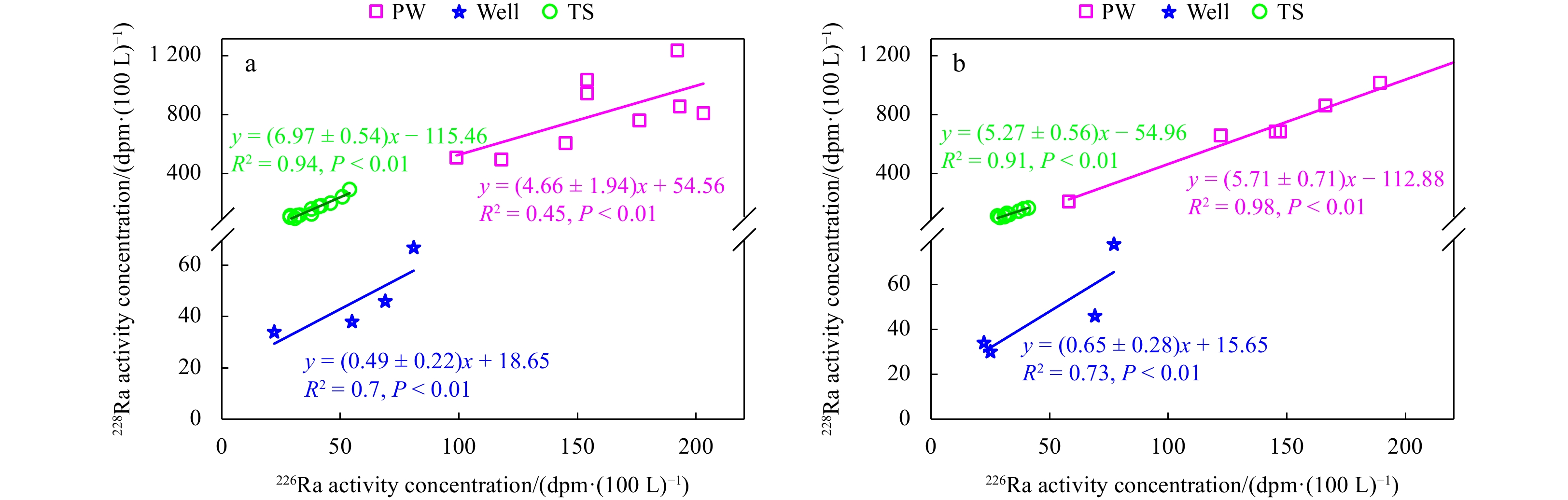
The salinity in the pore water around the ecozone ranged from 9.6 to 13.2 with an average of (11.7 ± 1.2) in the wet season, while it changed from 17.3 to 22.8 with an average of (21.4 ± 2.0) in the dry season (Table 1). The activities of pore water 222Rn and 228Ra varied greatly downstream along the coast of the mangrove creek in both seasons, from 1 240−4 630 Bq/m3 with an average of (2 670 ± 1 290) Bq/m3 for 222Rn and from 489−1 225 dpm/(100 L) with an average of (797 ± 245) dpm/(100 L) for 228Ra in the wet season, while from 1 410−5 130 Bq/m3 with an average of (3 080 ± 1 350) Bq/m3 for 222Rn and from 651−1 143 with an average of (744 ± 303) dpm/(100 L) for 228Ra in the dry season. The activity ratio of 228Ra to 226Ra, (228Ra/226Ra)AR of the pore water was (4.66 ± 1.94) in the wet season and slightly higher in the dry season (5.71 ± 0.71) (Fig. 2). On average, the pore water had a DIC concentration of (3 970 ± 1 400) µmol/L in the wet season and a few percents greater in the dry season. The concentration of DOC (µmol/L) was in the range from 206 to 425 with an average of (308 ± 65) in the wet season, and its average varied within 1% in the dry season. The properties of well water (fresh groundwater) were quite different from those of pore water. The activity of 222Rn was much greater in both seasons, about 20−30 times as much as that of pore water. However, the activity of 228Ra was only 7% equivalent to that of pore water. And the difference in (228Ra/226Ra)AR between the pore water and well water was also obvious. The (228Ra/226Ra)AR of the well water was (0.49 ± 0.22) and (0.65 ± 0.28) in the wet and dry seasons, respectively, which were much lower than that of the pore water (Fig. 2). In terms of the composition of dissolved carbon, the well water had a DIC concentration similar to the pore water, (4 098 ± 3 021) µmol/L in the wet season and (3 650 ± 611) µmol/L in the dry season, while its DOC concentration was an order of magnitude smaller than in the pore water in both seasons. The concentration of dissolved carbon of the Zhangjiang River water was the lowest in the carbon sources of the tidal creek, 628 µmol/L for DIC and 160 µmol/L for DOC in the dry season and about 100 µmol/L lower for DIC and 10 µmol/L lower for DOC in the wet season. The activities of 222Rn and 228Ra of the river water, 880 Bq/m3 and 41 dpm/(100 L) in the wet season and 610 Bq/m3 and 29 dpm/(100 L) in the dry season, were much lower than in the pore water. The value of (228Ra/226Ra)AR of the Zhangjiang River water was (1.41 ± 0.07) in the wet season and (1.49 ± 0.05) in the dry season. The seawater endmember had the lowest 222Rn activity concentration, 77 Bq/m3, in the wet season and remained the same order of magnitude in the dry season. The activity of 228Ra in the seawater varied from 181 dpm/(100 L) in the wet season to 154 dpm/(100 L) in the dry season. The concentration of DIC of the seawater endmember was a few times greater than in the river water, while the concentration of DOC was almost the same as in the river water (Table 1).
Table
1.
Sampling information and chemical parameters of the river water, seawater, sediments, well water, and pore water during the wet and dry seasons in the Zhangjiang River Estuary
Season
ID
Latitude
Longitude
Depth/m
Salinity
222Rn/ (Bq∙m−3)
226Ra/ (dpm∙(100 L)−1)
228Ra/ (dpm∙(100 L)−1)
DIC/ (μmol∙L−1)
TA/ (μmol∙L−1)
DOC (μmol∙L−1)
Wet season
PW 1
23.9270°N
117.4174°E
0.5
12.7
3070
203
802
5355
4061
359
PW 2
23.9270°N
117.4174°E
0.5
12.0
3070
193
847
6169
4336
343
PW 3
23.9261°N
117.4164°E
0.5
11.0
2210
176
750
3050
2605
258
PW 4
23.9259°N
117.4186°E
0.5
12.4
4630
154
1024
4023
3382
425
PW 5
23.9253°N
117.4186°E
0.5
11.0
1240
154
934
2784
2519
254
PW 6
23.9222°N
117.4233°E
0.5
13.2
1280
192
1225
4252
3916
323
PW 7
23.9158°N
117.4308°E
0.5
9.6
2350
99
501
2579
2383
315
PW 8
23.9317°N
117.4335°E
0.5
12.7
4600
118
489
5271
4706
288
PW 10
23.9253°N
117.4294°E
0.5
11.0
1620
145
600
2246
2129
206
Well 1
23.9247°N
117.4109°E
0
1.1
139000
81
67
6306
4173
46
Well 2
23.9204°N
117.4138°E
0
0.0
36700
55
38
1891
1168
11
SED 3
23.9261°N
117.4150°E
0.1
−
1280
−
−
−
−
−
SED 4
23.9261°N
117.4164°E
0.1
−
550
−
−
−
−
−
SED 6
23.9253°N
117.4186°E
0.1
−
543
−
−
−
−
−
SED 7
23.9222°N
117.4233°E
0.1
−
170
−
−
−
−
−
SED 10
23.9253°N
117.4294°E
0.1
−
543
−
−
−
−
−
ZJ
23.9528°N
117.3613°E
0
0.0
880
29
41
518
392
149
SW
23.9147°N
117.4706°E
0
20.1
77
63
181
1528
1623
154
Dry season
PW 1
23.9270°N
117.4174°E
0.5
17.3
4030
145
676
3061
2030
187
PW 3
23.9270°N
117.4164°E
0.5
22.0
1410
189
1005
3336
3104
465
PW 4
23.9261°N
117.4186°E
0.5
20.3
3830
147
677
5296
4767
322
PW 6
23.9259°N
117.4233°E
0.5
22.4
1580
224
1143
3507
3027
214
PW 7
23.9253°N
117.4308°E
0.5
22.8
2980
122
651
3121
2756
384
PW 8
23.9222°N
117.4335°E
0.5
22.3
5130
166
853
7577°N
7128°E
300
PW 10
23.9158°N
117.4294°E
0.5
22.6
2630
58
203
3033
2749
262
Well 1
23.9317°N
117.4109°E
0
0.9
111000
77
78
6775
3766
62
Well 2
23.9253°N
117.4138°E
0
0.0
37700
25
30
2138
1139
77
Well 3
23.9242°N
117.4128°E
0
0.0
33100
22
34
4205
2716
54
Well 4
23.9242°N
117.4136°E
0
0.0
112000
69
46
3116
1803
39
SED 3
23.9247°N
117.4150°E
0.1
−
737
−
−
−
−
−
SED 4
23.9204°N
117.4164°E
0.1
−
0
−
−
−
−
−
SED 5
23.9261°N
117.4186°E
0.1
−
373
−
−
−
−
−
SED 6
23.9261°N
117.4233°E
0.1
−
377
−
−
−
−
−
SED 7
23.9253°N
117.4294°E
0.1
−
373
−
−
−
−
−
SED 9
23.9158°N
117.4308°E
0.1
−
547
−
−
−
−
−
ZJ
23.9528°N
117.3613°E
0
0.0
610
19
29
628
658
160
SW
23.9147°N
117.4706°E
0
26.2
127
36
154
1939
2046
141
Note: PW represents pore water; Well, well water; SED, the interstitial water of sediments; ZJ, the Zhangjiang River endmember; and SW, the seawater endmember; DIC, dissolved inorganic concentration; DOC, dissolved organic concentration; TA, total alkalinity. 222Rn, 226Ra and 228Ra parameters indicate their activity concentrations. − represents no data.
Figure
2.
The activity concentration (1 Bq = 60 dpm) of 228Ra versus 226Ra at time series (TS) stations, in the well water and pore water (PW). a. Station TS1 in the wet season; b. Station TS2 in the dry season. Well represents the well water. The slope of the linear regression represents (228Ra/226Ra)AR. AR: activity ratio.
3.2
Time-series observations in the mangrove-dominated creek
During the 24-h observations at Station TS1, the tidal ranges in the wet season and the dry season were 2.5 m and 2.3 m, respectively. The salinity ranged from 2.0 to 8.2 in the wet season with no obvious pattern with water depth (Fig. 3a). In contrast, salinity varied in a greater range of 1.9−11.2 with a pattern more consistent with the variation of water depth in the dry season (Fig. 3b). The diurnal variation in temperature was greater in the wet season (25.2−35.3℃) than in the dry season (16.0−18.0℃). The activity of 222Rn dropped sharply during the flood tide from 797 Bq/m3 to 283 Bq/m3 and increased from 283 Bq/m3 to 437 Bq/m3 during the ebb tide in the wet season (Fig. 3a), whereas in the dry season it decreased from 603 Bq/m3 to 320 Bq/m3 during the flood flow and increased from 320 Bq/m3 to 827 Bq/m3 during the ebb flow (Fig. 3b).
Figure
3.
Time-series observations of temperature, salinity, water depth, 222Rn and 228Ra activity concentrations (1 Bq = 60 dpm), dissolved inorganic carbon (DIC), total alkalinity (TA), and dissolved organic carbone (DOC) concentrations, pCO2 (1 atm = 101 325 Pa) and the air-water CO2 flux $ {(F}_{{\mathrm{C}\mathrm{O}}_{2}}) $ at Stations TS1 and TS2. a and b are Station TS1 in the wet season and dry season, respectively, and c is Station TS2 in the dry season. Data are provided in Table S1.
Similar to the tidal pattern of 222Rn, the activity of 228Ra also mirrored the water depth varying from 91 dpm/(100 L) to 284 dpm/(100 L) in the wet season (Fig. 3a). The (228Ra/226Ra)AR in the mangrove-dominated creek in the wet season, (6.97 ± 0.54), was significantly higher than that of the well water, (0.49 ± 0.22), but similar to that of the pore water, (4.66 ± 1.94) (Fig. 2a). The tidal fluctuations of DIC and DOC concentrations showed trends similar to 222Rn and 228Ra in the wet season, with maximum DIC and DOC of 2 044 μmol/L and 468 μmol/L at the tidal trough and minimum DIC and DOC of 923 μmol/L and 247 μmol/L at the tidal crest (Fig. 3a). In the dry season, the concentrations of DIC and DOC followed similar tidal patterns with smaller diurnal variations, from 1 099−1 539 μmol/L for DIC and from 276−698 μmol/L for DOC (Fig. 3b). Meanwhile, pCO2 reached a peak value of 6 075 µatm at the lowest tide and a minimum value of 1 822 µatm at the highest tide in the wet season (Fig. 3a). In the dry season, the diel variation in pCO2 was relatively small from 1 878−4 940 µatm. The atmospheric pCO2 in the dry and wet seasons were 412 µatm and 388 µatm, respectively. Therefore, pCO2 in the creek far exceeded the atmospheric value in both wet and dry seasons, indicating that the tidal creek in the mangrove-dominated area was a strong source of atmospheric CO2. The average air pressure during September 2−4, 2018 was 100.5 kPa, while the average air pressure during March 9−11, 2019 was 101.1 kPa. The $ {F}_{{\mathrm{C}\mathrm{O}}_{2}} $ (mmol/(m2∙d)) was 0−27.9 with an average of (11.6 ± 8.7) in the wet season and 0.4−23.5 with a lower average of (9.5 ± 7.4) in the dry season. The diurnal pattern of $ {F}_{{\mathrm{C}\mathrm{O}}_{2}} $ in the two seasons differed from that of pCO2, but it still had a mirror relationship with the water depth (Figs 3a and b).
3.3
Time-series observations in the S. alterniflora-dominated creek
The diurnal variation in salinity at Station TS2 was from 1.3−9.3, which followed a pattern consistent with that in water depth, while the temperature with a diel range from 17.1℃ to 18.3℃ had no apparent trend. The activities of 222Rn and 228Ra varied with the same tidal pattern of decreasing with water depth. The diurnal change was from 227−760 Bq/m3 in 222Rn and 75−160 dpm/(100 L) in 228Ra (Fig. 3c). The (228Ra/226Ra)AR in the Spartina-dominated creek in the dry season, (5.27 ± 0.56), was significantly higher than that of the well water, (0.65 ± 0.28), but almost the same as that of the pore water, (5.71 ± 0.71) (Fig. 2b). The diel pattern of dissolved carbon was similar to that at Station TS1, with DIC in the range of 1 067−1 853 µmol/L and DOC in the range of 229−490 µmol/L (Fig. 3c). The diurnal variation in DIC at Station TS2 was 786 μmol/L, greater than its variation at Station TS1, while the diurnal change in DOC was 261 μmol/L. The $ {F}_{{\mathrm{C}\mathrm{O}}_{2}} $ mirrored the water depth with a maximum of 13.9 mmol/(m2∙d) and a minimum of 4.1 mmol/(m2∙d) (Fig. 3c). Compared with Station TS1, the variation of $ {F}_{{\mathrm{C}\mathrm{O}}_{2}} $ at Station TS2 almost followed the same pattern as that of pCO2, that is, decreasing during the flood tide and increasing during the ebb flow, in the range of 1 393−2 964 µatm (Fig. 3c).
3.4
Return flow factors in the tidal creeks
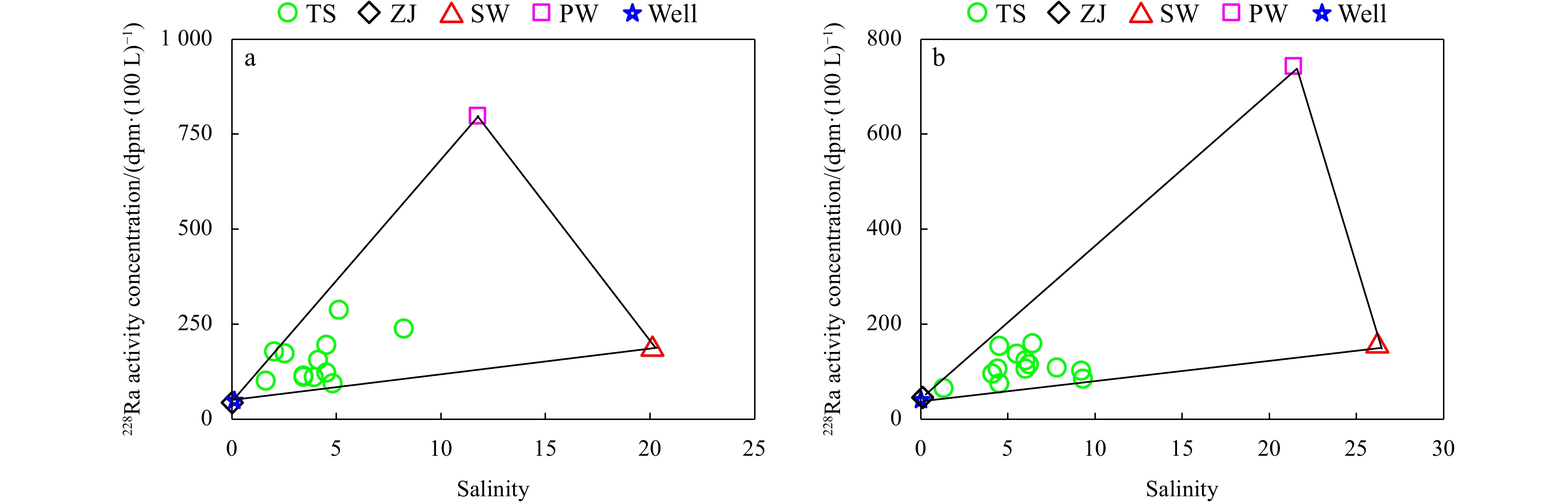
The flux of 228Ra from desorption from suspended particles was equivalent to 1% of that of rivers, 1%−3% of that of seawater, and less than 1% of that of pore water exchange. Therefore, the contribution from particle desorption can be ignored in the endmember mixing model. According to the distributions of 228Ra and salinity in the tidal creeks, three endmembers, seawater, the Zhangjiang River, and pore water were identified (Fig. 4). The proportion of seawater, i.e., the return flow factor, ranged from 2.7% to 28.9% in the mangrove-dominated creek in the wet season, and 0.3% to 33.8% in the Spartina-dominated creek in the dry season.
Figure
4.
The activity concentration of 228Ra (1 Bq = 60 dpm) versus salinity at the time series stations in the creeks, in the Zhangjiang River water, well water, seawater, and pore water. a. Station TS1 in the wet season; b. Station TS2 in the dry season. TS is the time series station, ZJ is the Zhangjiang River endmember, SW is the seawater endmember, PW is the pore water endmember, and Well is the well water.
3.5
Pore water exchange rates and associated carbon fluxes
In the mangrove-dominated creek (Station TS1), the pore water exchange rate in the wet season using the two tracers, 228Ra and 222Rn, was similar. The 222Rn-rate was [0, (9.0 ± 1.1)] cm/h with an integration rate over the observation period (24 h) of (82.1 ± 27.3) cm/d and the 228Ra-rate was [0, (9.2 ± 0.9)] cm/h with an integration rate of (77.4 ± 30.1) cm/d. The similarity of the two rates confirms the reliability of our calculations. Since the collection and determination of 222Rn are relatively convenient, our subsequent rate estimation in the dry season was based on 222Rn, which was [0, (13.6 ± 2.1)] cm/h with an integration rate of (110.0 ± 21.5) cm/d at Station TS1 and [0, (11.9 ± 2.1)] cm/h with an integration rate of (93.3 ± 50.2) cm/d in the Spartina-dominated creek (Station TS2). The rate fluctuated with the tide, with the minimum mostly occurring either at the tidal crest or the tidal trough in each tidal cycle (Fig. 5). Our pore water exchange rates are three orders of magnitude higher than that calculated by Wang et al. (2022). This discrepancy between our results and Wang et al. (2022) is caused by potentially great spatial differences in pore water exchange rates, different locations of sampling, and different methodology. Wang et al. (2022) adopted a direct observation of the change of water volume in two sediment pores with time to estimate the pore water exchange rate, one sediment pore was located in the salt marshes and the other was in the mangrove forest. In our study, we adopted an indirect method using radium and radon as the pore water exchange tracers to estimate the rate based on the changes of the tracers with time in the tidal creek. Apparently, the tidal creek received greater amount of pore water from surrounding pores in which many had much greater pore water exchange than those in Wang et al. (2022).
Figure
5.
Diurnal variation in the pore water exchange rate at Stations TS1 and TS2. a and b are the rates calculated using 222Rn and 228Ra in the wet season at Station TS1; c and d are the rates calculated using 222Rn in the dry season at Station TS1 and TS2.
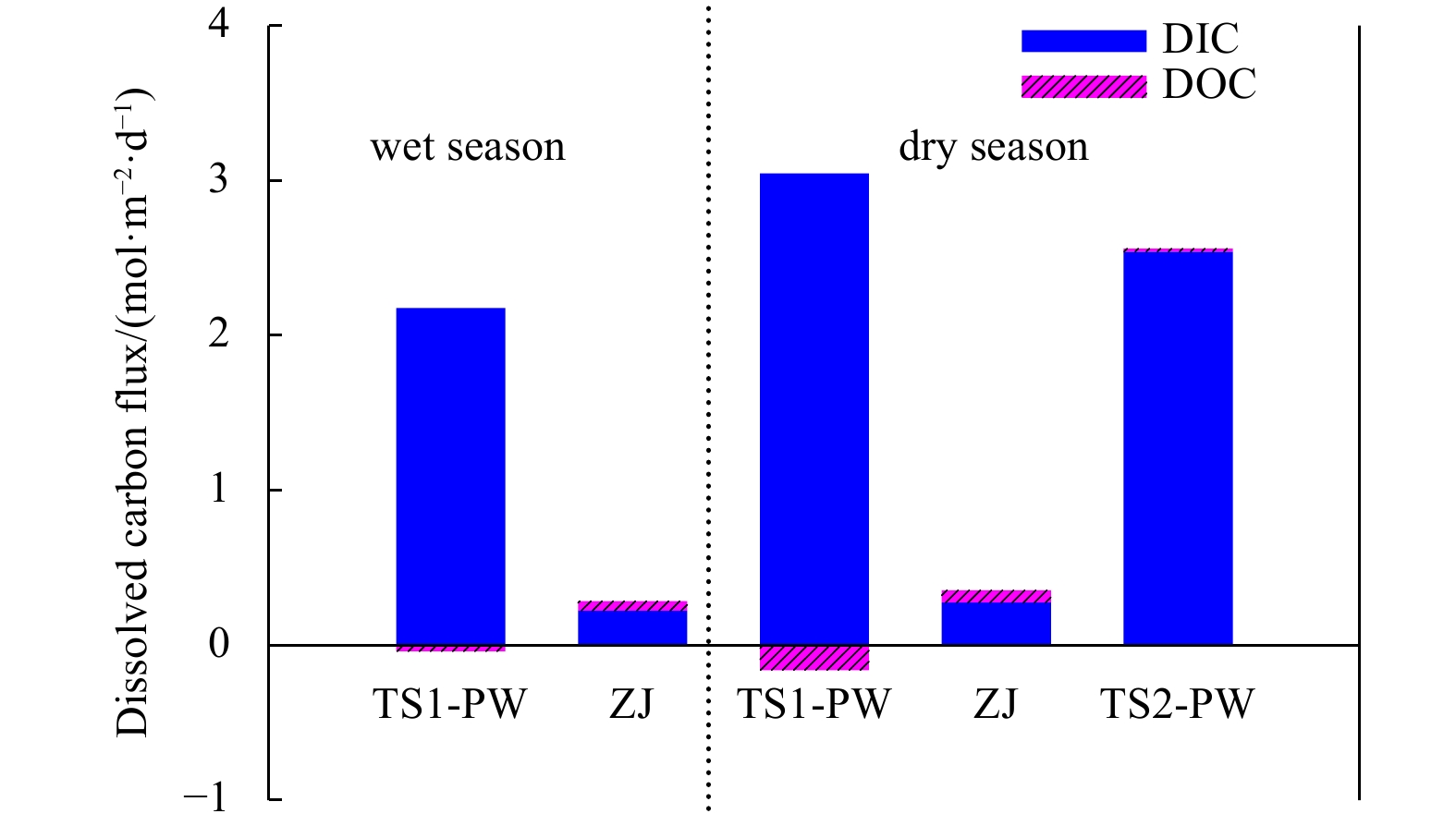
In the mangrove-dominated creek, the pore water exchange rate, (0.82 ± 0.27) m/d, was used to estimate the associated carbon flux in the wet season and (1.10 ± 0.22) m/d was used in the dry season. The associated carbon flux was (2.16 ± 0.63) mol/(m2∙d) for DIC and (–0.008 ± 0.07) mol/(m2∙d) for DOC in the wet season and (3.02 ± 0.65) mol/(m2∙d) for DIC and (−0.15 ± 0.007) mol/(m2∙d) for DOC in the dry season. The negative value means that pore water was a sink of DOC in the creek. The dissolved carbon (DC, the sum of DIC and DOC) flux via pore water exchange was (2.15 ± 0.63) mol/(m2∙d) in the wet season and (2.87 ± 0.65) mol/(m2∙d) in the dry season. In the S. alterniflora-dominated creek, using the pore water exchange rate of (0.93 ± 0.50) cm/d, less DIC, (2.52 ± 0.82) mol/(m2∙d), and DOC, (0.02 ± 0.09) mol/(m2∙d), inputs from the pore water occurred in the dry season, which resulted in a DC flux of (2.54 ± 0.82) mol/(m2∙d). The DC flux via pore water exchange was about 6−8 times greater than the riverine input in both seasons in the creeks of the mangrove-S. alterniflora ecozone (Fig. 6), indicating that pore water exchange was a much more important carbon source than the river.
Figure
6.
The dissolved carbon flux via pore water exchange in the mangrove-Spartina alterniflora ecozone in the Zhangjiang River Estuary in the dry and wet seasons. ZJ: Zhangjiang River; PW: pore water; TS: time series station; DIC: dissolved inorganic carbon; DOC: dissolved organic carbon.
The DIC flux via pore water exchange in the dry season was higher than in the wet season in the mangrove creek. This seasonal pattern differs from that in tropical Maowei Sea, where the estimated DIC flux was greater in the wet season as higher temperatures in the wet season, which can increase the activities of microbes to degrade more organic matter in mangrove soils and release larger amounts of DIC into aquifers (Chen et al., 2018). The reason for this difference is that the DIC flux via pore water exchange is determined not only by the concentration of the pore water endmember, but also by the pore water exchange rate. Although the DIC concentration of the pore water endmember in our system was slightly higher in the wet season (3 930 ± 1 410) than in the dry season (3 559 ± 870), the pore water exchange rate was higher in the dry season than in the wet season. The greater DIC flux via pore water exchange in the dry season in our system indicates that its seasonality was controlled more by the pore water exchange rate. Similarly, the DC flux was greater in the dry season than in the wet season.
3.6
Uncertainty analysis
The uncertainty in the pore water exchange rate was caused by the uncertainty in every other parameter in Eqs (1)−(18). Diffusion from sediments was taken as constant, so its contribution to the uncertainty in the pore water exchange rate was not evaluated. Here the uncertainties in h, t, λRn, T, and μ were taken as 0. The uncertainties in salinity, 222Rn, 228Ra, and carbon concentrations of the pore water endmember were the standard deviations of these parameters at multiple sites. Since there was only one sampling site for both the river water and sea water, the uncertainties of the above parameters of the river water and sea water were the measurement errors. Using error propagation (Text S1), the total uncertainty in the pore water exchange rate was mainly contributed by the uncertainty of 222Rn and 228Ra in the pore water endmember and the creek water (Table S2). For the radon-derived pore water exchange rate, the measurement error of radon was the largest source of uncertainty, while for the radium-derived pore water exchange rate, the largest uncertainty resulted from the spatial variation in the activity of 228Ra in the pore water endmember. The daily pore water exchange rate is the result of integrating the pore water exchange rate over the observation period (24 h), so the uncertainty of the daily rate we reported is the error propagated from the uncertainties of the discrete pore water exchange rates used in the integration.
The uncertainties in the net pore water exchange DIC and DOC fluxes resulted mainly from the uncertainty in the pore water exchange rate and the uncertainty in the carbon concentration of the pore water endmember, which represent the temporal variation in the pore water exchange rate and the spatial variation in the carbon concentration of the pore water endmember, respectively (Table S3). These uncertainties, however, would not change the conclusions reached based on the carbon fluxes calculated using the average chemical concentrations.
3.7
Contribution of pore water exchange to the air-water CO2flux in the tidal creeks
In the wet season, the average fraction of seawater, 0.13, in the mangrove-dominated creek, was taken in the calculation. In the dry season, the average return flow factor in the S. alterniflora-dominated creek, 0.15, was used for the ecozone. In the mangrove-dominated creek the pCO2 resulting from pore water exchange was 53% in the wet season and 71% in the dry season. The CO2 emission was 0−27.9 mmol/(m2∙d) (mean: (11.6 ± 8.7) mmol/(m2∙d)) in the wet season and 0.4−23.5 mmol/(m2∙d) (mean: (9.5 ± 7.4) mmol/(m2∙d)) in the dry season from the tidal creek. Pore water exchange contributed 75% of the CO2 emission in the wet season and 54% in the dry season. In the S. alterniflora-dominated creek, the CO2 emission in the dry season was 3.9−13.9 mmol/(m2∙d) (mean: (7.1 ± 2.7) mmol/(m2∙d)), 84% of which resulted from pore water exchange.
4.
Discussion
4.1
Pore water exchange rates in the tidal creeks of the mangrove-Spartina ecozone
4.1.1
Sources of water in the tidal creeks
Sediments in the ecozone are mainly silty clay up to 5−7 m deep, and mangrove roots exist within 90 cm of the ground surface (Lin, 2019), so freshwater groundwater below the sediments cannot have access to the tidal creeks. Similar low permeability of mangrove sediments has prevented fresh groundwater from entering the surface water in Florida Coastal Everglades (Whelan et al., 2005; Smith et al., 2016). The exclusion of fresh groundwater in the tidal creeks was further confirmed by (228Ra/226Ra)AR at the time-series stations and in the well waters (Fig. 2). The (228Ra/226Ra)AR in coastal waters is not affected by evaporation, precipitation, and biological activities, and is only controlled by physical mixing (Chen et al., 2010a; Krest et al., 1999; Nozaki et al., 1989). 226Ra (half-life of 1 600 a) and 228Ra (half-life of 5.75 a) are long-lived radium isotopes, with their half-lives much longer than the mixing time in coastal waters so that their decay is negligible. The (228Ra/226Ra)AR in the mangrove-dominated creek in the wet season was significantly different from that of the well water, but similar to that of the pore water (Fig. 2a). In the S. alterniflora creek, a similar pattern was observed (Fig. 2b). This indicates that the creek water in the ecozone had no obvious connection with the well water, instead the pore water was a potential source of radium for the creek water. The activity of 228Ra in the creeks apparently resulted from three endmembers, the river water, pore water and seawater (Fig. 4), which supports the three-endmember mixing model.
4.1.2
Seasonal and spatial variations of the pore water exchange rate in the ecozone
The pore water exchange rate was 30% higher in the dry season than in the wet season in the mangrove-dominated creek. Similar seasonal patterns were observed in other mangrove areas. For example, in the Shark River in Florida, USA, a mangrove-dominated estuary, the pore water exchange rate in the dry season was about three times as much as that in the wet season (Smith et al., 2016). The greater pore water exchange rate in the dry season coincided with a lower water level at the tidal trough in both systems.
In the same season, the pore water exchange rate in the mangrove-dominated creek was about 15% greater than in the S. alterniflora-dominated creek with a greater diurnal variation (Figs 5c, d). The greater exchange rate in the mangrove-dominated creek was likely caused by the following reasons: the dominant mangrove species in the Zhangjiang River Estuary were Avicennia marina, Kandelia candel, and paulownia trees, which average height was 2.3 m and their shading degree could reach more than 90%. The growth of large plant roots of mangroves could produce more routes of water infiltration (Meek et al., 1992). In addition, the lush mangroves provided food and shelter for the fiddler crabs that dig holes in the mangroves (Stieglitz et al., 2013). Their burrows have been observed to enhance the pore water exchange capacity in the Plum Island Estuary in Massachusetts, USA (Gardner and Gaines, 2008) and on Sapelo Island in GA, USA (Koretsky et al., 2002). At mangrove margins, however, where relatively sparsely distributed S. alterniflora invaded with mudflats exposed, the vegetation coverage was much less than in the mangrove-dominated area (Feng et al., 2017) and the depth and density of caves formed by crabs decreased (Wang et al., 2014), which resulted in lower pore water exchange rate in the Spartina-dominated creek.
4.1.3
Global comparison of the pore water exchange rate
In terms of mangroves and salt marshes, our pore water exchange rates in the ecozone fall within the range of global pore water exchange/submairine groundwater discharge rates, 0−990 cm/d, in coastal wetlands (Susilo et al., 2005; Prakash et al., 2018; Santos et al., 2021). To take global mangrove systems, in particular, for comparison, mangroves with different coastline types were summarized (Table 2). Based on the statistics of 2016, the global mangrove area is about 1.38×10⁵ km2, mainly distributed in the tropical area (Alongi, 2014; Chen et al., 2018), 40.5% of which is delta, 27.5% is estuary, 21.0% is open coast, and the left (11.0%) is lagoon according to the classification proposed by Worthington et al. (2020). Pore water exchange rates vary greatly in different regions, but on the whole, the rates in deltaic and estuarine mangroves are greater than those in lagoonal and open coast mangroves. The Zhangjiang River Estuary mangrove is an estuarine system, and its pore water exchange rate is at least a few time greater than that in lagoonal mangrove systems. Similar magnitude of pore water exchange was also observed in other mangrove-dominated estuaries (Table 2). Mangrove roots and biological activities, such as fiddler crabs, made densely distributed holes on both sides of the tidal creeks, which resulted in intensive pore water exchange (Stieglitz et al., 2013). These results indicate that although the low permeability of the mangrove peats prohibited fresh groundwater from entering the tidal creeks, great fluid exchange was still present due to the densely distributed burrows (Hemond and Fifield, 1982; Stieglitz et al., 2000; Wilson and Gardner, 2006; Xin et al., 2009, 2013).
Table
2.
Pore water exchange rates and carbon storage in different types of mangrove systems around the globe
4.2
Local importance of pore water exchange to the air-water CO2emission
As CO2 released by pore water exchange equilibrates usually within tens of seconds with bicarbonate ion in the creek water (Pilson, 2013), a simple multiplication of the pore water exchange rate and the CO2 concentration in the pore water is not what the pore water exchange really contributes to the air-sea CO2 flux. How much of the air-sea CO2 flux in mangrove tidal creeks directly resulting from pore water exchange has seldom been accurately quantified.
The observation in the mangrove-dominated creek shows that the tidal creek is the hot spot of CO2 emission in the mangrove system in both wet and dry seasons, as observed in other mangrove systems (Kristensen et al., 2008; Taillardat et al., 2018; Call et al., 2019), and the air-water CO2 exchange flux of tidal creek in our study area is low in the global mangroves (Table 2). Furthermore, the contribution of pore water exchange to the CO2 emission flux in the tidal creek is more than 50% than that in both seasons, which proves that pore water exchange is the main driving factor of air-water CO2 flux in the mangrove tidal creek (Chen et al., 2021b). This also means that these carbon, which is believed to have been stored in the soil for thousands of years (Page et al., 2002), will be re-discharged to coastal waters via pore water exchange, and then returned to the atmosphere through air-water interface exchange.
In addition, the daily average air-water CO2 flux in the S. alterniflora-dominated creek was 20% lower than in the mangrove-dominated creek (Fig. S1a). With the same water temperature, salinity, wind speed, and air pressure used in the flux calculation at the two stations in the creeks, the difference in the air-water CO2 fluxes between the two stations was mainly caused by the difference in pCO2 in the tidal creeks as the pCO2 in the S. alterniflora-dominated creek was lower by 32% than in the mangrove-dominated creek (Fig. 3). As pore water exchange was a main regulator of pCO2 in the tidal creeks, we infer that the less emission in the S. alterniflora-dominated creek was mainly caused by the relatively weak pore water exchange (Fig. S1b).
4.3
Importance of pore water exchange to the lateral carbon transport
To estimate the lateral carbon transport in the creeks, carbon outwelling was estimated by integration over a diel cycle of the product of the carbon concentration and the water flow (Maher et al., 2013). Since the Zhangjiang River had a relatively small discharge and the creeks were dominated by tidal flows, the same water depth was ensured at the beginning and end of the integration period. The results showed that in the mangrove-dominated creek, there was a net export downstream of DIC (1.87 mol/(m2∙d)) and DOC (0.42 mol/(m2∙d)) in the wet season. In the dry season, the tidal creek exported greater DC downstream with 2.34 mol/(m2∙d) for DIC and 0.54 mol/(m2∙d) for DOC. The carbon carried by the pore water exchange in the form of DIC accounted for 100% of the DIC outwelling from the tidal creek. In the DC outwelling about 80% was in form of DIC in both seasons. This is similar to the results in the tidal creek of Evans head, Australia (Santos et al., 2019). In the S. alterniflora-dominated creek, an outwelling of DC of 2.88 mol/(m2∙d) occurred in the dry season, which included 3.17 mol/(m2∙d) for DIC and −0.29 mol/(m2∙d) for DOC, indicating that the DC outwelling was 100% in the form of DIC. Similar to the mangrove-dominated creek, the DC transported by the pore water exchange in the form of DIC accounted for 79% of the DIC outwelling from the tidal creek. Our results indicate that most of the carbon carried by the pore water exchange into the creeks was exported to the ocean in the form of DIC under the pumping of tides. We highlight that since only one day measurements have been carried out in each creek, and there was only one station in each landscape, it was impossible to draw a statistical conclusion. But the difference between the two stations still indicates that the invasion of S. alterniflora may have changed the fate of carbon fixed in the intertidal wetlands.
4.4
The role of pore water exchange in the fate of the carbon fixed by the mangrove-Spartina alterniflora system
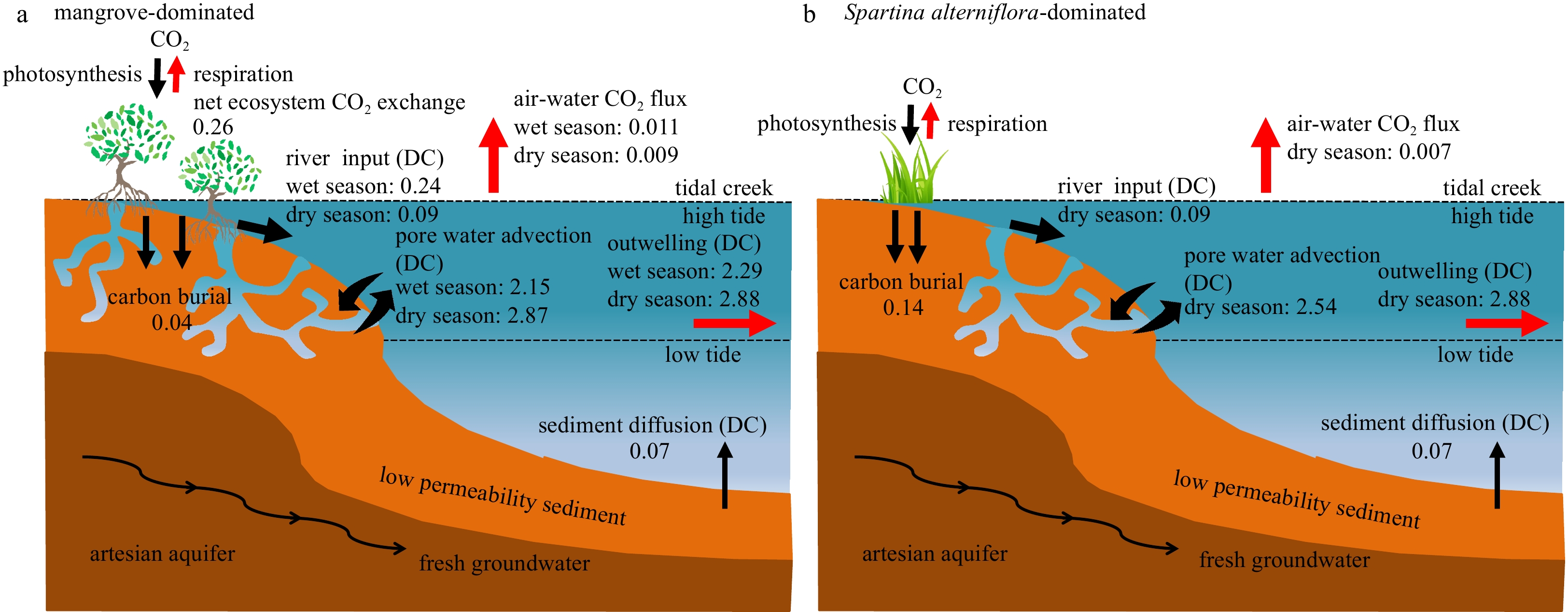
To evaluate the impact of net carbon export from soils via pore water exchange into the creeks of the mangrove-S. alterniflora ecozone, we compiled the known carbon sources and sinks of the system and set up a conceptual framework of the fate of carbon fixed by the vegetations in the ecozone as follows (Fig. 7). The vegetation absorbs carbon in the form of CO2 from the atmosphere through photosynthesis. Some of the fixed carbon is respired by the vegetation to CO2 and directly released back to the atmosphere, while the other fixed carbon is stored in the vegetation or buried in the soil or exported via pore water exchange. The DIC fluxes via pore water exchange were greater than the DOC fluxes, suggesting that DIC was the main form of carbon exported by pore water exchange (Fig. 6), which confirms the missing mangrove carbon sink being the pore water-exported DIC (Maher et al., 2013). Note that the pore water exchange occurs in the tidal creeks, while the net primary production and carbon accretion in the mangrove system are intended for the whole mangrove-covered region. The soil carbon accretion is a net result of gross carbon burial in the soil and pore water exchange. The total area of tidal creeks in the mangroves of the ecozone is about 2.87×10⁴ m2, while the total mangrove-covered area is 5.74×10⁵ m2 (Fig. 1). The carbon via pore water exchange in the tidal creeks of the mangrove system, calculated as the carbon flux via pore water exchange multiplied by the total area of the tidal creeks, was (6.17×10⁴−8.23×10⁴) mol/d. The net carbon fixed by mangrove vegetation was estimated with the net ecosystem CO2 exchange, 0.26 mol/(m2∙d) (Zhu et al., 2021), multiplied by the total mangrove-covered area, to be 1.49×10⁵ mol/d. The amount of soil carbon accretion was 2.29×10⁴ mol/d, calculated with the mangrove-covered area multiplied by the soil carbon accretion rate of 0.04 mol/(m2∙d) (Chen et al., 2021a). Thus, the carbon via pore water exchange in the tidal creeks of the mangrove system accounted for 41%−55% of the net carbon fixed by mangrove vegetation and 3−4 times as much as the soil carbon accretion. Less than 5% of the carbon exported from the soil via pore water exchange is released in the form of CO2 from the creeks as the pCO2 in the creeks increases due to the DIC addition from pore water exchange. The DIC exported from soils via pore water accounts for 79%−100% of the DIC outwelling into the estuary from the mangrove-S. alterniflora ecozone. The results confirm that a major export pathway for carbon from mangroves is through root and soil respiration and subsequent dissolved inorganic carbon export via pore water (Alongi, 2014, 2020). The residence time of DIC (mostly as alkalinity) in the ocean is about 100 000 a (Santos et al., 2019; Yau et al., 2022), making DIC outwelling from the mangrove-S. alterniflora ecozone a long-term storage mechanism for the carbon fixed by the mangroves and S. alterniflora in addition to burial in the soil. Similarly, in the mangrove creeks in Australia (Maher et al., 2013) and Vietnam (Taillardat et al., 2018), pore water exchange traced by radon can explain nearly 100% of the DIC outwelling. Such a great carbon loss term in the subtropical mangrove-Spartina ecozone of the Zhangjiang River Estuary confirms that the ability of the blue carbon habitat to effectively fix carbon has been highly underestimated as observed in other mangroves (Maher et al., 2018). Globally, only about 13% of the carbon absorbed by mangrove vegetation via photosynthesis has been deposited in the soil (Alongi, 2014). Therefore, quantification of the pore water exchange and related soil carbon loss is essential to fully understand their carbon fixation capacity.
Figure
7.
Schematic diagram of the fate of carbon in the mangrove-Spartina alterniflora ecozone in the Zhangjiang River Estuary. a. The mangrove-dominated area; b. the S. alterniflora-dominated area. The soil carbon deposition rates in the mangrove-dominated and the S. alterniflora-dominated areas are from Chen et al. (2021a). The sediment dissolved carbon diffusion flux data are from Chen et al. (2018). The net ecosystem CO2 exchange data in mangrove system are from Zhu et al. (2021). The unit is in mol/(m2∙d). DC: dissolved carbon (the sum of DIC and DOC) flux.
In this study, we quantified the dissolved carbon flux via pore water exchange and assessed the fate of the exported carbon in the mangrove-Spartina ecozone in the Zhangjiang River Estuary, China. The dissolved carbon flux based on the mass balance of 222Rn and 228Ra was (2.15 ± 0.63) mol/(m2∙d) in the wet season and (2.87 ± 0.65) mol/(m2∙d) in the dry season in the mangrove-dominated creek and 11% lower in the S. alterniflora-dominated creek, which was about 6−8 times greater than the riverine input in both seasons in the tidal creeks of the ecozone. The smaller export of dissolved carbon from soils via pore water exchange in the S. alterniflora-dominated creek implies similar occurrence likely in other regions where S. alterniflora invades. The pore water exchange in the ecozone contributed 54%−84% of the emission of CO2 from the tidal creeks. The dissolved carbon exported from soils via pore water exchange to the tidal creeks were found to be in the form of DIC, which accounted for all of the DIC outwelling from the mangrove-dominated creek and 79% of the DIC outwelling from the S. alterniflora creek.
Acknowledgements:
We express our sincere gratitude to Captain Zhaorong Wang from Zhangzhou, Fujian Province, China for his assistance in collecting the pore water samples. We also extend our gratitude to the two anonymous reviewers for all their constructive comments which helped improving the quality of manuscript.
Adame M F, Kauffman J B, Medina I, et al. 2013. Carbon stocks of tropical coastal wetlands within the karstic landscape of the Mexican Caribbean. PLoS ONE, 8(2): e56569. doi: 10.1371/journal.pone.0056569
Alongi D M. 2012. Carbon sequestration in mangrove forests. Carbon Management, 3(3): 313–322. doi: 10.4155/cmt.12.20
Alongi D M. 2014. Carbon cycling and storage in mangrove forests. Annual Review of Marine Science, 6: 195–219. doi: 10.1146/annurev-marine-010213-135020
Alongi D M. 2020. Carbon balance in salt marsh and mangrove ecosystems: a global synthesis. Journal of Marine Science and Engineering, 8(10): 767. doi: 10.3390/jmse8100767
Alongi D M, Tirendi F, Dixon P, et al. 1999. Mineralization of organic matter in intertidal sediments of a tropical semi-enclosed delta. Estuarine, Coastal and Shelf Science, 48(4): 451–467,
Alongi D M, Trott L A, Rachmansyah, et al. 2008. Growth and development of mangrove forests overlying smothered coral reefs, Sulawesi and Sumatra, Indonesia. Marine Ecology Progress Series, 370: 97–109. doi: 10.3354/meps07661
Alongi D M, Wattayakorn G, Pfitzner J, et al. 2001. Organic carbon accumulation and metabolic pathways in sediments of mangrove forests in southern Thailand. Marine Geology, 179(1–2): 85–103,
Arias-Ortiz A, Masqué P, Glass L, et al. 2021. Losses of soil organic carbon with deforestation in mangroves of Madagascar. Ecosystems, 24(1): 1–19. doi: 10.1007/S10021-020-00500-Z
Atwood T B, Connolly R M, Almahasheer H, et al. 2017. Global patterns in mangrove soil carbon stocks and losses. Nature Climate Change, 7(7): 523–528. doi: 10.1038/NCLIMATE3326
Bianchi T S, Allison M A, Zhao Jun, et al. 2013. Historical reconstruction of mangrove expansion in the Gulf of Mexico: linking climate change with carbon sequestration in coastal wetlands. Estuarine, Coastal and Shelf Science, 119: 7–16,
Biswas H, Mukhopadhyay S K, De T K, et al. 2004. Biogenic controls on the air-water carbon dioxide exchange in the Sundarban mangrove environment, northeast coast of Bay of Bengal, India. Limnology and Oceanography, 49(1): 95–101. doi: 10.4319/lo.2004.49.1.0095
Borges V A, Djenidi S, Lacroix G, et al. 2003. Atmospheric CO2 flux from mangrove surrounding waters. Geophysical Research Letters, 30(11): 1558. doi: 10.1029/2003GL017143
Bouillon S, Borges A V, Castañeda-Moya E, et al. 2008. Mangrove production and carbon sinks: a revision of global budget estimates. Global Biogeochemical Cycles, 22(2): GB2013. doi: 10.1029/2007GB003052
Bouillon S, Frankignoulle M, Dehairs F, et al. 2003. Inorganic and organic carbon biogeochemistry in the Gautami Godavari Estuary (Andhra Pradesh, India) during pre-monsoon: the local impact of extensive mangrove forests. Global Biogeochemical Cycles, 17(4): 1114. doi: 10.1029/2002GB002026
Brunskill G J, Zagorskis I, Pfitzner J. 2002. Carbon burial rates in sediments and a carbon mass balance for the Herbert River region of the great barrier reef continental shelf, North Queensland, Australia. Estuarine, Coastal and Shelf Science, 54(4): 677–700,
Burnett W C, Dulaiova H. 2003. Estimating the dynamics of groundwater input into the coastal zone via continuous radon-222 measurements. Journal of Environmental Radioactivity, 69(1–2): 21–35,
Burnett W C, Peterson R, Moore W S, et al. 2008. Radon and radium isotopes as tracers of submarine groundwater discharge—Results from the Ubatuba, Brazil SGD assessment intercomparison. Estuarine, Coastal and Shelf Science, 76(3): 501–511,
Call M, Maher D T, Santos I R, et al. 2015. Spatial and temporal variability of carbon dioxide and methane fluxes over semi-diurnal and spring–neap–spring timescales in a mangrove creek. Geochimica et Cosmochimica Acta, 150: 211–225. doi: 10.1016/j.gca.2014.11.023
Call M, Santos I R, Dittmar T, et al. 2019. High pore-water derived CO2 and CH4 emissions from a macro-tidal mangrove creek in the Amazon region. Geochimica et Cosmochimica Acta, 247: 106–120. doi: 10.1016/j.gca.2018.12.029
Chen Siming. 2021. Potential distribution of Spartina alterniflora along the Chinese coast and its response to climate change. Journal of Ecology and Rural Environment (in Chinese), 37(12): 1575–1585. doi: 10.19741/j.issn.1673-4831.2021.0509
Chen Luzhen, Chen Yining, Zhang Yihui, et al. 2021a. Mangrove carbon sequestration and sediment deposition changes under cordgrass invasion. In: Sidik F, Friess D A, eds. Dynamic Sedimentary Environments of Mangrove Coasts. Amsterdam: Elsevier Press, 473–509
Chen Weifang, Liu Qian, Huh C A, et al. 2010a. Signature of the Mekong River plume in the western South China Sea revealed by radium isotopes. Journal of Geophysical Research: Oceans, 115(C12): C12002. doi: 10.1029/2010JC006460
Chen Xiaogang, Santos I R, Call M, et al. 2021b. The mangrove CO2 pump: tidally driven pore-water exchange. Limnology and Oceanography, 66(4): 1563–1577. doi: 10.1002/lno.11704
Chen Guangchen, Ulumuddin Y I, Pramudji S, et al. 2014. Rich soil carbon and nitrogen but low atmospheric greenhouse gas fluxes from North Sulawesi mangrove swamps in Indonesia. Science of the Total Environment, 487: 91–96. doi: 10.1016/j.scitotenv.2014.03.140
Chen Juan, Wu Feihua, Xiao Qiang, et al. 2010b. Diurnal variation of nitric oxide emission flux from a mangrove wetland in Zhangjiang River Estuary, China. Estuarine, Coastal and Shelf Science, 90(4): 212–220,
Chen Xiaogang, Zhang Fenfen, Lao Yanling, et al. 2018. Submarine groundwater discharge-derived carbon fluxes in mangroves: an important component of blue carbon budgets?. Journal of Geophysical Research: Oceans, 123(9): 6962–6979. doi: 10.1029/2018JC014448
Choi Y, Wang Yang. 2004. Dynamics of carbon sequestration in a coastal wetland using radiocarbon measurements. Global Biogeochemical Cycles, 18(4): GB4016. doi: 10.1029/2004GB002261
Corbett D R, Burnett W C, Cable P H, et al. 1998. A multiple approach to the determination of radon fluxes from sediments. Journal of Radioanalytical and Nuclear Chemistry, 236(1–2): 247–253,
Cusack M, Saderne V, Arias-Ortiz A, et al. 2018. Organic carbon sequestration and storage in vegetated coastal habitats along the western coast of the Arabian Gulf. Environmental Research Letters, 13(7): 074007. doi: 10.1088/1748-9326/aac899
Donato D C, Kauffman J B, Murdiyarso D, et al. 2011. Mangroves among the most carbon-rich forests in the tropics. Nature Geoscience, 4(5): 293–297. doi: 10.1038/NGEO1123
Feng Jianxiang, Zhou Jian, Wang Liming, et al. 2017. Effects of short-term invasion of Spartina alterniflora and the subsequent restoration of native mangroves on the soil organic carbon, nitrogen and phosphorus stock. Chemosphere, 184: 774–783. doi: 10.1016/j.chemosphere.2017.06.060
Gao Guifeng, Li Pengfei, Shen Zhijun, et al. 2018. Exotic Spartina alterniflora invasion increases CH4 while reduces CO2 emissions from mangrove wetland soils in southeastern China. Scientific Reports, 8(1): 9243. doi: 10.1038/s41598-018-27625-5
Gardner L R, Gaines E F. 2008. A method for estimating pore water drainage from marsh soils using rainfall and well records. Estuarine, Coastal and Shelf Science, 79(1): 51–58,
Gonneea M E, Paytan A, Herrera-Silveira J A. 2004. Tracing organic matter sources and carbon burial in mangrove sediments over the past 160 years. Estuarine, Coastal and Shelf Science, 61(2): 211–227,
Grellier S, Janeau J L, Nhon D H, et al. 2017. Changes in soil characteristics and C dynamics after mangrove clearing (Vietnam). Science of the Total Environment, 593–594: 654–663,
Hamilton S E, Friess D A. 2018. Global carbon stocks and potential emissions due to mangrove deforestation from 2000 to 2012. Nature Climate Change, 8(3): 240–244. doi: 10.1038/s41558-018-0090-4
Hemond H F, Fifield J L. 1982. Subsurface flow in salt marsh peat: a model and field study. Limnology and Oceanography, 27(1): 126–136. doi: 10.4319/lo.1982.27.1.0126
Henry K M, Twilley R R. 2013. Soil development in a coastal Louisiana wetland during a climate-induced vegetation shift from salt marsh to mangrove. Journal of Coastal Research, 29(6): 1273–1283. doi: 10.2112/JCOASTRES-D-12-00184.1
Jones T G, Ratsimba H R, Ravaoarinorotsihoarana L, et al. 2014. Ecological variability and carbon stock estimates of mangrove ecosystems in northwestern Madagascar. Forests, 5(1): 177–205. doi: 10.3390/f5010177
Kauffman J B, Trejo H H, del Carmen Jesus Garcia M, et al. 2016. Carbon stocks of mangroves and losses arising from their conversion to cattle pastures in the Pantanos de Centla, Mexico. Wetlands Ecology and Management, 24(2): 203–216. doi: 10.1007/s11273-015-9453-z
Kelly J L, Dulai H, Glenn C R, et al. 2019. Integration of aerial infrared thermography and in situ radon-222 to investigate submarine groundwater discharge to Pearl Harbor, Hawaii, USA. Limnology and Oceanography, 64(1): 238–257. doi: 10.1002/lno.11033
Koné Y J M, Borges A V. 2008. Dissolved inorganic carbon dynamics in the waters surrounding forested mangroves of the Ca Mau Province (Vietnam). Estuarine, Coastal and Shelf Science, 77(3): 409–421,
Konikow L F, Akhavan M, Langevin C D, et al. 2013. Seawater circulation in sediments driven by interactions between seabed topography and fluid density. Water Resources Research, 49(3): 1386–1399. doi: 10.1002/wrcr.20121
Koretsky C M, Meile C, Van Cappellen P. 2002. Quantifying bioirrigation using ecological parameters: a stochastic approach. Geochemical Transactions, 3(1): 17. doi: 10.1186/1467-4866-3-17
Krest J M, Moore W S, Rama. 1999. 226Ra and 228Ra in the mixing zones of the Mississippi and Atchafalaya Rivers: indicators of groundwater input. Marine Chemistry, 64(3): 129–152. doi: 10.1016/S0304-4203(98)00070-X
Kristensen E, Flindt M R, Ulomi S, et al. 2008. Emission of CO2 and CH4 to the atmosphere by sediments and open waters in two Tanzanian mangrove forests. Marine Ecology Progress Series, 370: 53–67. doi: 10.3354/meps07642
Kusumaningtyas M A, Hutahaean A A, Fischer H W, et al. 2019. Variability in the organic carbon stocks, sources, and accumulation rates of Indonesian mangrove ecosystems. Estuarine, Coastal and Shelf Science, 218: 310–323,
Lambert M J, Burnett W C. 2003. Submarine groundwater discharge estimates at a Florida coastal site based on continuous radon measurements. Biogeochemistry, 66(1–2): 55–73,
Li Dongyi, Xu Yonghang, Li Yunhai, et al. 2018. Sedimentary records of human activity and natural environmental evolution in sensitive ecosystems: a case study of a coral nature reserve in Dongshan Bay and a mangrove forest nature reserve in Zhangjiang River Estuary, Southeast China. Organic Geochemistry, 121: 22–35. doi: 10.1016/j.orggeochem.2018.02.011
Lin Qiulian. 2019. The influence of aerial root/belowground root structure on the vertical accretion and elevation change of mangroves (in Chinese)[dissertation]. Xiamen: Xiamen University
Liu Mingyue, Li Huiying, Li Lin, et al. 2017. Monitoring the invasion of Spartina alterniflora using multi-source high-resolution imagery in the Zhangjiang Estuary, China. Remote Sensing, 9(6): 539. doi: 10.3390/rs9060539
Lynch J C, Meriwether J R, McKee B A, et al. 1989. Recent accretion in mangrove ecosystems based on 137Cs and 210Pb. Estuaries, 12(4): 284–299. doi: 10.2307/1351907
MacIntyre S, Wanninkhof R H, Chanton J P. 1995. Trace gas exchange across the air-water interface in freshwater and coastal marine environments. In: Mattson P A, Harris R C, eds. Methods in Ecology-Biogenic Trace Gases: Measuring Emissions from Soil and Water. New York: Blackwell Science, 52–77
MacKenzie R, Sharma S, Rovai A R. 2021. Environmental drivers of blue carbon burial and soil carbon stocks in mangrove forests. In: Sidik F, Friess D A, eds. Dynamic Sedimentary Environments of Mangrove Coasts. Amsterdam: Elsevier Press, 275–294
Maher D T, Call M, Santos I R, et al. 2018. Beyond burial: lateral exchange is a significant atmospheric carbon sink in mangrove forests. Biology Letters, 14(7): 20180200. doi: 10.1098/rsbl.2018.0200
Maher D T, Santos I R, Golsby-Smith L, et al. 2013. Groundwater-derived dissolved inorganic and organic carbon exports from a mangrove tidal creek: the missing mangrove carbon sink?. Limnology and Oceanography, 58(2): 475–488. doi: 10.4319/lo.2013.58.2.0475
Maher D T, Santos I R, Schulz K G, et al. 2017. Blue carbon oxidation revealed by radiogenic and stable isotopes in a mangrove system. Geophysical Research Letters, 44(10): 4889–4896. doi: 10.1002/2017GL073753
Martens C S, Kipphut G W, Val Klump J. 1980. Sediment-water chemical exchange in the coastal zone traced by in situ radon-222 flux measurements. Science, 208(4441): 285–288. doi: 10.1126/science.208.4441.285
Meek B D, Rechel E R, Carter L M, et al. 1992. Infiltration rate of a sandy loam soil: effects of traffic, tillage, and plant roots. Soil Science Society of America Journal, 56(3): 908–913. doi: 10.2136/sssaj1992.03615995005600030038x
Millero F J, Hiscock W T, Huang F, et al. 2001. Seasonal variation of the carbonate system in Florida Bay. Bulletin of Marine Science, 68(1): 101–123
Monji N, Hamotani K, Hamada Y, et al. 2002. Exchange of CO2 and heat between mangrove forest and the atmosphere in wet and dry seasons in southern Thailand. Journal of Agricultural Meteorology, 58(2): 71–77. doi: 10.2480/agrmet.58.71
Moore W S, Arnold R. 1996. Measurement of 223Ra and 224Ra in coastal waters using a delayed coincidence counter. Journal of Geophysical Research: Oceans, 101(C1): 1321–1329. doi: 10.1029/95JC03139
Moore W S, Blanton J O, Joye S B. 2006. Estimates of flushing times, submarine groundwater discharge, and nutrient fluxes to Okatee Estuary, South Carolina. Journal of Geophysical Research: Oceans, 111(C9): C09006. doi: 10.1029/2005JC003041
Nozaki Y, Kasemsupaya V, Tsubota H. 1989. Mean residence time of the shelf water in the East China and the Yellow Seas determined by 228Ra/226Ra measurements. Geophysical Research Letters, 16(11): 1297–1300. doi: 10.1029/gl016i011p01297
Page S E, Siegert F, Rieley J O, et al. 2002. The amount of carbon released from peat and forest fires in Indonesia during 1997. Nature, 420(6911): 61–65. doi: 10.1038/nature01131
Passos T R G, Artur A G, Nóbrega G N, et al. 2016. Comparison of the quantitative determination of soil organic carbon in coastal wetlands containing reduced forms of Fe and S. Geo-Marine Letters, 36(3): 223–233. doi: 10.1007/s00367-016-0437-7
Pelletier L, Strachan I B, Roulet N T, et al. 2015. Can boreal peatlands with pools be net sinks for CO2?. Environmental Research Letters, 10(3): 035002. doi: 10.1088/1748-9326/10/3/035002
Peng T H, Takahashi T, Broecker W S. 1974. Surface radon measurements in the North Pacific Ocean Station Papa. Journal of Geophysical Research, 79(12): 1772–1780. doi: 10.1029/JC079i012p01772
Pilson M E Q. 2013. An Introduction to the Chemistry of the Sea. 2nd ed. Cambridge: Cambridge University, 396–398
Prakash R, Srinivasamoorthy K, Gopinath S, et al. 2018. Radon isotope assessment of submarine groundwater discharge (SGD) in Coleroon River Estuary, Tamil Nadu, India. Journal of Radioanalytical and Nuclear Chemistry, 317(1): 25–36. doi: 10.1007/s10967-018-5877-2
Pülmanns N, Diele K, Mehlig U, et al. 2014. Burrows of the semi-terrestrial crab Ucides cordatus enhance CO2 release in a north Brazilian mangrove forest. PLoS ONE, 9(10): e109532. doi: 10.1371/journal.pone.0109532
Ranjan R K, Routh J, Ramanathan A L, et al. 2011. Elemental and stable isotope records of organic matter input and its fate in the Pichavaram mangrove-estuarine sediments (Tamil Nadu, India). Marine Chemistry, 126(1–4): 163–172,
Ray R, Ganguly D, Chowdhury C, et al. 2011. Carbon sequestration and annual increase of carbon stock in a mangrove forest. Atmospheric Environment, 45(28): 5016–5024. doi: 10.1016/j.atmosenv.2011.04.074
Ray R, Michaud E, Aller R C, et al. 2018. The sources and distribution of carbon (DOC, POC, DIC) in a mangrove dominated estuary (French Guiana, South America). Biogeochemistry, 138(3): 297–321. doi: 10.1007/s10533-018-0447-9
Reithmaier G M S, Chen Xiaogang, Santos I R, et al. 2021. Rainfall drives rapid shifts in carbon and nutrient source-sink dynamics of an urbanised, mangrove-fringed estuary. Estuarine Coastal and Shelf Science, 249: 107064. doi: 10.1016/j.ecss.2020.107064
Ridd P V. 1996. Flow through animal burrows in mangrove creeks. Estuarine, Coastal and Shelf Science, 43(5): 617–625,
Robinson C, Li L, Barry D A. 2007. Effect of tidal forcing on a subterranean estuary. Advances in Water Resources, 30(4): 851–865. doi: 10.1016/j.advwatres.2006.07.006
Rovai A S, Twilley R R. 2021. Gaps, challenges, and opportunities in mangrove blue carbon research: a biogeographic perspective. In: Sidik F, Friess D A, eds. Dynamic Sedimentary Environments of Mangrove Coasts. Amsterdam: Elsevier Press, 295–334
Rovai A S, Twilley R R, Castañeda-Moya E, et al. 2018. Global controls on carbon storage in mangrove soils. Nature Climate Change, 8(6): 534–538. doi: 10.1038/s41558-018-0162-5
Sanders C J, Maher D T, Tait D R, et al. 2016. Are global mangrove carbon stocks driven by rainfall?. Journal of Geophysical Research: Biogeosciences, 121(10): 2600–2609. doi: 10.1002/2016JG003510
Sanders C J, Santos I R, Barcellos R, et al. 2012. Elevated concentrations of dissolved Ba, Fe and Mn in a mangrove subterranean estuary: consequence of sea level rise?. Continental Shelf Research, 43: 86–94. doi: 10.1016/j.csr.2012.04.015
Sanders C J, Smoak J M, Naidu A S, et al. 2010. Mangrove forest sedimentation and its reference to sea level rise, Cananeia, Brazil. Environmental Earth Sciences, 60(6): 1291–1301. doi: 10.1007/s12665-009-0269-0
Santos I R, Chen Xiaogang, Lecher A L, et al. 2021. Submarine groundwater discharge impacts on coastal nutrient biogeochemistry. Nature Reviews Earth & Environment, 2(5): 307–323. doi: 10.1038/s43017-021-00152-0
Santos I R, Maher D T, Eyre B D. 2012. Coupling automated radon and carbon dioxide measurements in coastal waters. Environmental Science & Technology, 46(14): 7685–7691. doi: 10.1021/es301961b
Santos I R, Maher D T, Larkin R, et al. 2019. Carbon outwelling and outgassing vs. burial in an estuarine tidal creek surrounded by mangrove and saltmarsh wetlands. Limnology and Oceanography, 64(3): 996–1013. doi: 10.1002/lno.11090
Seeberg-Elverfeldt J, Schlüter M, Feseker T, et al. 2005. Rhizon sampling of porewaters near the sediment-water interface of aquatic systems. Limnology and Oceanography: Methods, 3(8): 361–371. doi: 10.4319/lom.2005.3.361
Smith C G, Price R M, Swarzenski P W, et al. 2016. The role of ocean tides on groundwater-surface water exchange in a mangrove-dominated estuary: shark river slough, Florida Coastal Everglades, USA. Estuaries and Coasts, 39(6): 1600–1616. doi: 10.1007/s12237-016-0079-z
Stieglitz T C, Clark J F, Hancock G J. 2013. The mangrove pump: the tidal flushing of animal burrows in a tropical mangrove forest determined from radionuclide budgets. Geochimica et Coshmochimica Acta, 102: 12–22. doi: 10.1016/j.gca.2012.10.033
Stieglitz T, Ridd P, Müller P. 2000. Passive irrigation and functional morphology of crustacean burrows in a tropical mangrove swamp. Hydrobiologia, 421(1): 69–76. doi: 10.1023/A:1003925502665
Susilo A, Ridd P V, Thomas S. 2005. Comparison between tidally driven groundwater flow and flushing of animal burrows in tropical mangrove swamps. Wetlands Ecology and Management, 13(4): 377–388. doi: 10.1007/s11273-004-0164-0
Swarzenski P, Reich C, Rudnick D. 2009. Examining submarine ground-water discharge into Florida bay by using 222Rn and continuous resistivity profiling. U. S. Geological Survey, Open-File Report 2008–1342. https://pubs.usgs.gov/publication/ofr20081342[2009-07-0-23/2022-09-08]
Sweeney C, Gloor E, Jacobson A R, et al. 2007. Constraining global air-sea gas exchange for CO2 with recent bomb 14C measurements. Global Biogeochemical Cycles, 21(2): GB2015. doi: 10.1029/2006GB002784
Taillardat P, Willemsen P, Marchand C, et al. 2018. Assessing the contribution of porewater discharge in carbon export and CO2 evasion in a mangrove tidal creek (Can Gio, Vietnam). Journal of Hydrology, 563: 303–318. doi: 10.1016/j.jhydrol.2018.05.042
Tait D R, Maher D T, Macklin P A, et al. 2016. Mangrove pore water exchange across a latitudinal gradient. Geophysical Research Letters, 43(7): 3334–3341. doi: 10.1002/2016GL068289
Tait D R, Maher D T, Sanders C J, et al. 2017. Radium-derived porewater exchange and dissolved N and P fluxes in mangroves. Geochimica et Cosmochimica Acta, 200: 295–309. doi: 10.1016/j.gca.2016.12.024
Tateda Y, Nhan D D, Wattayakorn G, et al. 2005. Preliminary evaluation of organic carbon sedimentation rates in Asian mangrove coastal ecosystems estimated by 210Pb chronology. Radioprotection, 40(S1): S527–S532. doi: 10.1051/radiopro:2005s1-077
Thompson B S, Clubbe C P, Primavera J H, et al. 2014. Locally assessing the economic viability of blue carbon: a case study from Panay Island, the Philippines. Ecosystem Services, 8: 128–140. doi: 10.1016/j.ecoser.2014.03.004
Wang Mao, Gao Xueqin, Wang Wenqing. 2014. Differences in burrow morphology of crabs between Spartina alterniflora marsh and mangrove habitats. Ecological Engineering, 69: 213–219. doi: 10.1016/j.ecoleng.2014.03.096
Wang Fenfang, Xiao Kai, Santos I R, et al. 2022. Porewater exchange drives nutrient cycling and export in a mangrove-salt marsh ecotone. Journal of Hydrology, 606: 127401. doi: 10.1016/j.jhydrol.2021.127401
Wanninkhof R. 1992. Relationship between wind speed and gas exchange over the ocean. Journal of Geophysical Research: Oceans, 97(C5): 7373–7382. doi: 10.1029/92JC00188
Weiss R F. 1974. Carbon dioxide in water and seawater: the solubility of a non-ideal gas. Marine Chemistry, 2(3): 203–215. doi: 10.1016/0304-4203(74)90015-2
Whelan K R T, Smith T J, Cahoon D R, et al. 2005. Groundwater control of mangrove surface elevation: shrink and swell varies with soil depth. Estuaries, 28(6): 833–843. doi: 10.1007/BF02696013
Wilson A M, Gardner L R. 2006. Tidally driven groundwater flow and solute exchange in a marsh: numerical simulations. Water Resources Research, 42(1): W01405. doi: 10.1029/2005WR004302
Worthington T A, Zu Ermgassen P S E, Friess D A, et al. 2020. A global biophysical typology of mangroves and its relevance for ecosystem structure and deforestation. Scientific Reports, 10(1): 14652. doi: 10.1038/s41598-020-71194-5
Xin Pei, Jin Guangqiu, Li Ling, et al. 2009. Effects of crab burrows on pore water flows in salt marshes. Advances in Water Resources, 32(3): 439–449. doi: 10.1016/j.advwatres.2008.12.008
Xin Pei, Li Ling, Barry D A. 2013. Tidal influence on soil conditions in an intertidal creek-marsh system. Water Resources Research, 49(1): 137–150. doi: 10.1029/2012WR012290
Yando E S, Osland M J, Willis J M, et al. 2016. Salt marsh-mangrove ecotones: using structural gradients to investigate the effects of woody plant encroachment on plant-soil interactions and ecosystem carbon pools. Journal of Ecology, 104(4): 1020–1031. doi: 10.1111/1365-2745.12571
Yau Y Y Y, Xin Pei, Chen Xiaogang, et al. 2022. Alkalinity export to the ocean is a major carbon sequestration mechanism in a macrotidal saltmarsh. Limnology and Oceanography, 67(S2): S158–S170. doi: 10.1002/lno.12155
Zhang Yan, Li Hailong, Wang Xuejing, et al. 2016. Estimation of submarine groundwater discharge and associated nutrient fluxes in eastern Laizhou Bay, China using 222Rn. Journal of Hydrology, 533: 103–113. doi: 10.1016/j.jhydrol.2015.11.027
Zhang Ruifeng, Yan Chongling, Liu Jingchun. 2013. Effect of mangroves on the horizontal and vertical distributions of rare earth elements in sediments of the Zhangjiang Estuary in Fujian Province, southeastern China. Journal of Coastal Research, 29(6): 1341–1350. doi: 10.2112/JCOASTRES-D-11-00215.1
Zhu Xudong, Sun Chenyang, Qin Zhangcai. 2021. Drought-induced salinity enhancement weakens mangrove greenhouse gas cycling. Journal of Geophysical Research: Biogeosciences, 126(8): e2021JG006416. doi: 10.1029/2021JG006416
Jian’an Liu, Xueqing Yu, Xinyi Lin, et al. The importance of porewater exchange process on carbon lateral export from saltmarsh creek to coastal sea. Journal of Oceanology and Limnology, 2024. doi:10.1007/s00343-024-3261-3
2.
Jing Zhou, Jinzhou Du, Kaijun Su, et al. Substantially excess uranium in the waters of an intertidal salt marsh: A case study of eastern Chongming Beach. Estuarine, Coastal and Shelf Science, 2023. doi:10.1016/j.ecss.2023.108585
Weizhen Jiang, Guizhi Wang, Qing Li, Manab Kumar Dutta, Shilei Jin, Guiyuan Dai, Yi Xu. The fate of carbon resulting from pore water exchange in a mangrove and Spartina alterniflora ecozone[J]. Acta Oceanologica Sinica, 2023, 42(8): 61-76. doi: 10.1007/s13131-023-2234-2
Weizhen Jiang, Guizhi Wang, Qing Li, Manab Kumar Dutta, Shilei Jin, Guiyuan Dai, Yi Xu. The fate of carbon resulting from pore water exchange in a mangrove and Spartina alterniflora ecozone[J]. Acta Oceanologica Sinica, 2023, 42(8): 61-76. doi: 10.1007/s13131-023-2234-2
Table
1.
Sampling information and chemical parameters of the river water, seawater, sediments, well water, and pore water during the wet and dry seasons in the Zhangjiang River Estuary
Season
ID
Latitude
Longitude
Depth/m
Salinity
222Rn/ (Bq∙m−3)
226Ra/ (dpm∙(100 L)−1)
228Ra/ (dpm∙(100 L)−1)
DIC/ (μmol∙L−1)
TA/ (μmol∙L−1)
DOC (μmol∙L−1)
Wet season
PW 1
23.9270°N
117.4174°E
0.5
12.7
3070
203
802
5355
4061
359
PW 2
23.9270°N
117.4174°E
0.5
12.0
3070
193
847
6169
4336
343
PW 3
23.9261°N
117.4164°E
0.5
11.0
2210
176
750
3050
2605
258
PW 4
23.9259°N
117.4186°E
0.5
12.4
4630
154
1024
4023
3382
425
PW 5
23.9253°N
117.4186°E
0.5
11.0
1240
154
934
2784
2519
254
PW 6
23.9222°N
117.4233°E
0.5
13.2
1280
192
1225
4252
3916
323
PW 7
23.9158°N
117.4308°E
0.5
9.6
2350
99
501
2579
2383
315
PW 8
23.9317°N
117.4335°E
0.5
12.7
4600
118
489
5271
4706
288
PW 10
23.9253°N
117.4294°E
0.5
11.0
1620
145
600
2246
2129
206
Well 1
23.9247°N
117.4109°E
0
1.1
139000
81
67
6306
4173
46
Well 2
23.9204°N
117.4138°E
0
0.0
36700
55
38
1891
1168
11
SED 3
23.9261°N
117.4150°E
0.1
−
1280
−
−
−
−
−
SED 4
23.9261°N
117.4164°E
0.1
−
550
−
−
−
−
−
SED 6
23.9253°N
117.4186°E
0.1
−
543
−
−
−
−
−
SED 7
23.9222°N
117.4233°E
0.1
−
170
−
−
−
−
−
SED 10
23.9253°N
117.4294°E
0.1
−
543
−
−
−
−
−
ZJ
23.9528°N
117.3613°E
0
0.0
880
29
41
518
392
149
SW
23.9147°N
117.4706°E
0
20.1
77
63
181
1528
1623
154
Dry season
PW 1
23.9270°N
117.4174°E
0.5
17.3
4030
145
676
3061
2030
187
PW 3
23.9270°N
117.4164°E
0.5
22.0
1410
189
1005
3336
3104
465
PW 4
23.9261°N
117.4186°E
0.5
20.3
3830
147
677
5296
4767
322
PW 6
23.9259°N
117.4233°E
0.5
22.4
1580
224
1143
3507
3027
214
PW 7
23.9253°N
117.4308°E
0.5
22.8
2980
122
651
3121
2756
384
PW 8
23.9222°N
117.4335°E
0.5
22.3
5130
166
853
7577°N
7128°E
300
PW 10
23.9158°N
117.4294°E
0.5
22.6
2630
58
203
3033
2749
262
Well 1
23.9317°N
117.4109°E
0
0.9
111000
77
78
6775
3766
62
Well 2
23.9253°N
117.4138°E
0
0.0
37700
25
30
2138
1139
77
Well 3
23.9242°N
117.4128°E
0
0.0
33100
22
34
4205
2716
54
Well 4
23.9242°N
117.4136°E
0
0.0
112000
69
46
3116
1803
39
SED 3
23.9247°N
117.4150°E
0.1
−
737
−
−
−
−
−
SED 4
23.9204°N
117.4164°E
0.1
−
0
−
−
−
−
−
SED 5
23.9261°N
117.4186°E
0.1
−
373
−
−
−
−
−
SED 6
23.9261°N
117.4233°E
0.1
−
377
−
−
−
−
−
SED 7
23.9253°N
117.4294°E
0.1
−
373
−
−
−
−
−
SED 9
23.9158°N
117.4308°E
0.1
−
547
−
−
−
−
−
ZJ
23.9528°N
117.3613°E
0
0.0
610
19
29
628
658
160
SW
23.9147°N
117.4706°E
0
26.2
127
36
154
1939
2046
141
Note: PW represents pore water; Well, well water; SED, the interstitial water of sediments; ZJ, the Zhangjiang River endmember; and SW, the seawater endmember; DIC, dissolved inorganic concentration; DOC, dissolved organic concentration; TA, total alkalinity. 222Rn, 226Ra and 228Ra parameters indicate their activity concentrations. − represents no data.
Note: PER: pore water exchange rate; SCD: soil carbon density; CAR: carbon accretion rate. − represents no data.
Figure 1. Study area and sampling stations. a. Location of the study site; b. the sampling stations; c. the stations in the tidal creeks; d. the mangrove-dominated area (Station TS1); e. the Spartina alterniflora-dominated area (Station TS2).
Figure 2. The activity concentration (1 Bq = 60 dpm) of 228Ra versus 226Ra at time series (TS) stations, in the well water and pore water (PW). a. Station TS1 in the wet season; b. Station TS2 in the dry season. Well represents the well water. The slope of the linear regression represents (228Ra/226Ra)AR. AR: activity ratio.
Figure 3. Time-series observations of temperature, salinity, water depth, 222Rn and 228Ra activity concentrations (1 Bq = 60 dpm), dissolved inorganic carbon (DIC), total alkalinity (TA), and dissolved organic carbone (DOC) concentrations, pCO2 (1 atm = 101 325 Pa) and the air-water CO2 flux $ {(F}_{{\mathrm{C}\mathrm{O}}_{2}}) $ at Stations TS1 and TS2. a and b are Station TS1 in the wet season and dry season, respectively, and c is Station TS2 in the dry season. Data are provided in Table S1.
Figure 4. The activity concentration of 228Ra (1 Bq = 60 dpm) versus salinity at the time series stations in the creeks, in the Zhangjiang River water, well water, seawater, and pore water. a. Station TS1 in the wet season; b. Station TS2 in the dry season. TS is the time series station, ZJ is the Zhangjiang River endmember, SW is the seawater endmember, PW is the pore water endmember, and Well is the well water.
Figure 5. Diurnal variation in the pore water exchange rate at Stations TS1 and TS2. a and b are the rates calculated using 222Rn and 228Ra in the wet season at Station TS1; c and d are the rates calculated using 222Rn in the dry season at Station TS1 and TS2.
Figure 6. The dissolved carbon flux via pore water exchange in the mangrove-Spartina alterniflora ecozone in the Zhangjiang River Estuary in the dry and wet seasons. ZJ: Zhangjiang River; PW: pore water; TS: time series station; DIC: dissolved inorganic carbon; DOC: dissolved organic carbon.
Figure 7. Schematic diagram of the fate of carbon in the mangrove-Spartina alterniflora ecozone in the Zhangjiang River Estuary. a. The mangrove-dominated area; b. the S. alterniflora-dominated area. The soil carbon deposition rates in the mangrove-dominated and the S. alterniflora-dominated areas are from Chen et al. (2021a). The sediment dissolved carbon diffusion flux data are from Chen et al. (2018). The net ecosystem CO2 exchange data in mangrove system are from Zhu et al. (2021). The unit is in mol/(m2∙d). DC: dissolved carbon (the sum of DIC and DOC) flux.


 DownLoad:


 DownLoad:


 DownLoad: