Hyperspectral remote sensing identification of marine oil emulsions based on the fusion of spatial and spectral features

1. Introduction

A marine oil spill is an unexpected event at sea and an important target of marine environmental monitoring. In recent years, marine oil spills, such as the 2018 East China Sea Sanchi oil spill, the 2020 Mauritius offshore cargo ship oil spill, and the 2021 Yellow Sea Symphony oil spill, have occurred frequently, causing serious harm to the marine environment. Marine oil spills form oil-in-water (OW) and water-in-oil (WO) emulsions under the action of wind, waves, and other marine environmental dynamics (Hu et al., 2021). Compared with floating crude oil on the sea surface, oil emulsions are difficult to recover, and the pollution in the environment is not easy to eliminate. Monitoring marine oil spill emulsion is a key task in oil spill emergency response. Synthetic aperture radar (SAR) and optical remote sensing are important technologies for marine oil spill monitoring. Marine oil emulsions reduce the surface roughness and weaken the backscattering of satellite microwave radar signals from the oil spill surface, which can be detected by SAR. However, the low wind speed area and the upwelling area on the sea surface result in similar dark pixel features in SAR images, which interfere with the identification of oil emulsions. Optical remote sensing can use spectral features to identify and quantitatively invert different types of oil emulsions, but it is affected by weather. In addition, the spectrum of oil emulsions changes because of different water content, and emulsions are often mixed and distributed with floating crude oil on the sea surface. Thus, the use of remote sensing to accurately identify oil emulsions remains a challenging research topic.

In recent years, the optical remote sensing of marine oil emulsions has made great progress. Leifer et al. studied the spectra of different types and concentrations of oil emulsions (Leifer et al., 2012). Lu et al. (2016, 2020) analyzed the spectral characteristics of different types of oil emulsions and their response mechanisms, and showed that oil emulsions exhibit significant -C-H bond absorption at 1200 nm, 1730 nm and 2370 nm. On the basis of the relationship between the volume concentration of oil emulsions and their reflection spectra, the feasibility of using optical remote sensing for oil spill emulsion identification and quantitative inversion was analyzed (Lu et al., 2016, 2020). With the rapid development of machine learning techniques, research on marine oil spill identification based on machine learning and hyperspectral imaging has gradually progressed. Li et al. used different machine learning algorithms to identify marine oil spill types under simulated marine environment conditions, and the results showed that machine learning can effectively extract the features in the hyperspectral data of oil spills and improve the accuracy of oil spill type identification (Li et al., 2021; Xie et al., 2022). Although the rich waveband information of hyperspectral data can help target identification, it also causes information redundancy, resulting in reduced classification accuracy and efficiency, and even overfitting in machine learning models (Su, 2022; Jiang and Ma, 2020). Studies have shown that spectral feature selection can effectively enhance the identification of targets from hyperspectral data (Zhang, 2016). For example, a spectral feature selection method based on functional group feature detection has been used to accurately distinguish between marine oil spills and Sargassum in hyperspectral images (Shi et al., 2018); the use of spectral standard deviation analysis and factor analysis has also been used to effectively identify typical oil types in marine oil spills (Yang et al., 2021). Nonetheless, the current research on marine oil spill identification based on hyperspectral and deep learning mainly focuses on oil spill detection, oil type identification, and oil film thickness inversion, and less research is conducted on the identification of different types of oil spill emulsions. Jiao et al. (2022) used an experimentally constructed HSV model to identify different types of oil spill emulsions. However, in practice, the value of the hue threshold in this method needs to be adjusted on the basis of different application scenarios (Jiao et al., 2022). Using the spatial-spectral features of hyperspectral data images, the development of deep learning-based methods for the identification of oil spill emulsions can fully exploit the spatial spectrum information of remote sensing data, which should improve the identification accuracy of oil spill emulsions (Fauvel et al., 2013; Du et al., 2022).

Here, a spectral feature selection method based on the standard deviation (SD) threshold and mutual information (MI) is established for OW and WO spill emulsions. Using the oil spill hyperspectral data acquired in the outdoor simulated ocean environment, the characteristic bands that can distinguish between crude oil, OW, WO and seawater are extracted, and an oil spill emulsion identification model that fuses spatial and spectral features is established. Using oil spill airborne hyperspectral data, we conducted identification experiments on oil spill emulsions in different background waters and under different spatial and temporal conditions, analyzed the transferability of the model, and explored the effects of feature band selection and spectral resolution on the identification of marine oil spill emulsions.

2. Data acquisition and analysis

2.1 Airborne oil spill hyperspectral data

2.1.1   Airborne hyperspectral remote sensing data for outfield experiments

The spectral responses of different types of oil spill emulsions differ significantly. To clarify the characteristics of oil spill emulsions in the visible-short-wave infrared range and then carry out the remote sensing identification of marine oil spill emulsions, we designed an outfield oil-spill airborne hyperspectral observation experiment. An inflatable pool of 10 m × 10 m was placed in the Qingdao Marina, and the pool was divided into four compartments using a barrier. The four compartments were filled with seawater, and then laboratory-prepared WO emulsion with 80% volume concentration, OW emulsion with 0.1% volume concentration, and crude oil samples were each injected into one of the compartments. The occurrence of emulsification in marine oil spills is indeed influenced by the composition of the oil. When the oil contains a certain amount of hydrocarbons, it is more prone to forming stable emulsions with water (Zhong and You, 2011). The wax and asphaltene contents in the crude oil used in this study are 7.56% and 1.57%, respectively, capable of forming stable emulsions with water. After multiple preparations in the laboratory and reference to other experiments involving the preparation of oil emulsions (Lu et al., 2019), we found that WO emulsion with 80% volume concentration and OW emulsion with 0.1% volume concentration are stable and exhibit absorption features of the -C-H and -O-H bonds in the oil. This makes them representative and suitable as observation targets for outfield experiments.

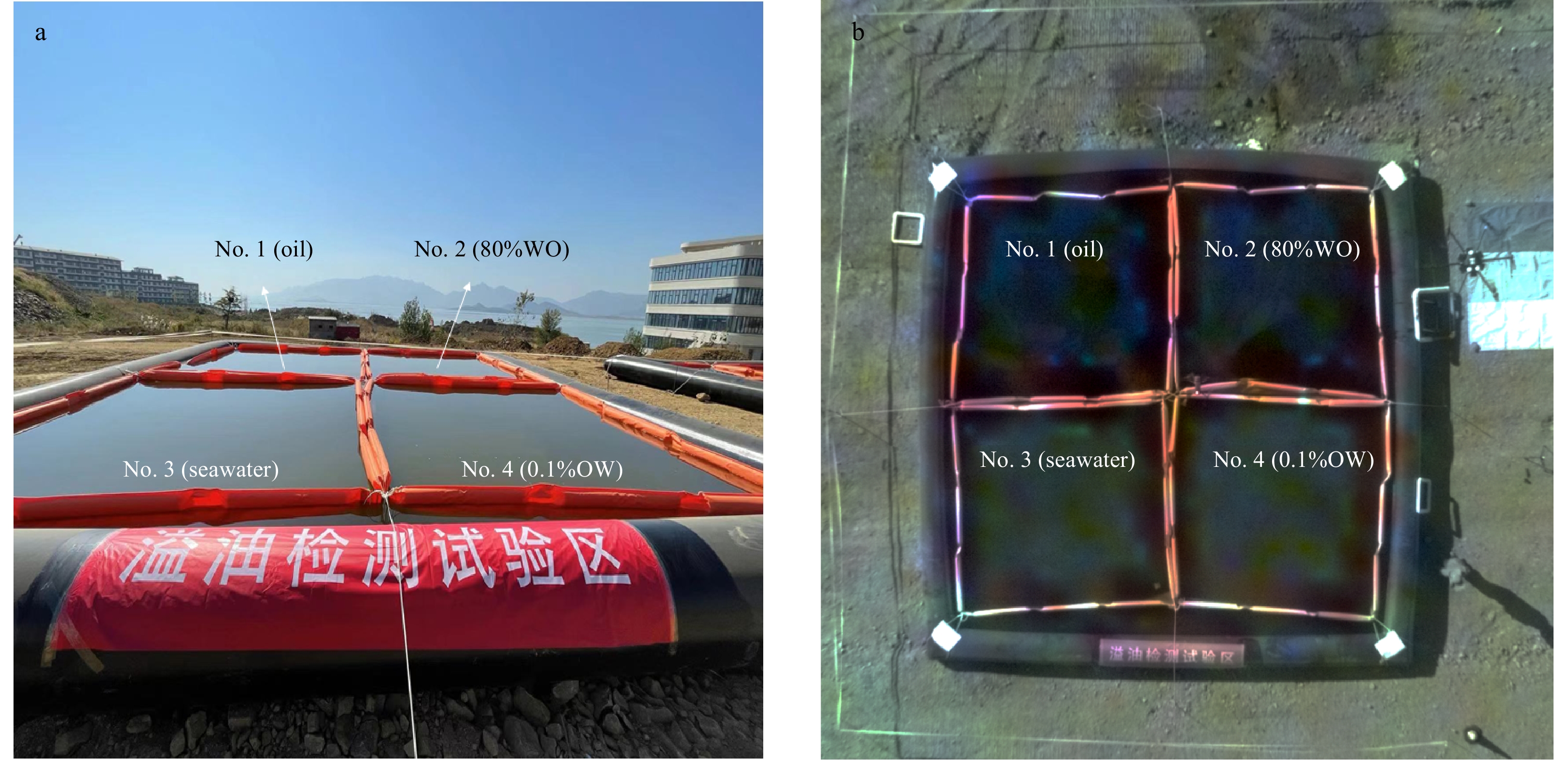
The unmanned Cubert S185 hyperspectral imager was used to acquire the target observation data, and an unmanned aerial vehicle equipped with a 4K sensor was used for simultaneous observation. The Cubert S185 sensor has a band range of 450–950 nm, a spectral resolution of 4 nm, a total of 126 bands, and an instantaneous field of view of 23°. The flight height of the unmanned aerial vehicle in the experiment was 40 m, and the spatial resolution of the image pixels was 0.016 m. Scenes of the experimental setup are shown in Fig. 1.

Figure  1.  Setup of the experiments for the airborne hyperspectral observation of marine oil spills. a. Outfield oil spill hyperspectral observation experimental setup. b. Experimentally acquired S185 airborne hyperspectral image, true color composite: red: 638 nm, green: 550 nm, blue: 472 nm. The pool was divided into four enclosures injected with seawater. No. 1 was injected with crude oil, No. 2 was injected with WO at 80% volume concentration, No. 3 contained pure seawater and No. 4 was injected with OW at 0.1% volume concentration.

DownLoad: Full-Size Img PowerPoint

2.1.2   Airborne hyperspectral remote sensing data of a typical oil spill incident

The hyperspectral image data acquired by the Airborne Visible Infrared Imaging Spectrometer (AVIRIS) during the 2010 oil spill in the US Gulf of Mexico were used to conduct oil spill emulsion identification experiments. The data pre-processing included atmospheric correction, removal of the atmospheric absorption bands, and spectral normalization. The original image contained 224 bands, and 160 bands remained after removing the atmospheric absorption bands. The three selected study areas are shown in Fig. 2. The data in study area 1 were used to train the oil spill and emulsion identification model, and the data from study area 2 were used to test the model’s spatial migration performance, i.e., the model trained on study area 1 was used to identify the oil spill and its emulsion in study area 2, and the performance of the model at different locations was also evaluated. The data from study area 3 were used to test the spatial and temporal migration of the model, i.e., the trained model was used to identify the oil spill and its emulsions in study area 3 and test the model’s effectiveness in identifying the oil spill and its emulsions under different spatial and temporal conditions.

Figure  2.  US Gulf of Mexico May 2010 AVIRIS true color composite image. For the subgraph located on the upper side, the study area overlaid on a MODIS image on 17 May 2010, true color composite. Study areas 1 and 2 were selected from the AVIRIS r10 image on 18 May 2010, and study area 3 was selected from an r11 image on 17 May 2010, true color composite: red: 638 nm, green: 550 nm, blue: 472 nm. Study area 1 is used for model training, study area 2 is used to evaluate the model’s spatial migration performance, and study area 3 is used to evaluate its spatial and temporal migration.

DownLoad: Full-Size Img PowerPoint

2.2 Outfield land-based hyperspectral data acquisition and analysis

Seawater can be categorized into two types of water bodies, Class Ⅰ and Class Ⅱ, according to their optical properties. A typical Class Ⅰ water body is the open ocean water body, which is low in suspended solids. Class Ⅱ water body contains more suspended matter and soluble organic compound and thus shows reflection peaks in the visible band. In the identification of marine oil spill remote sensing images, it is necessary to consider the influence of different background water bodies on the identification results, so we carried out oil emulsion identification experiments for both Class Ⅰ and Class Ⅱ water bodies. In this study, hyperspectral data of WO at 60%–90% by volume, OW at 0.1% by volume, seawater, and crude oil samples were acquired in an outfield simulated marine environment using an Analytical Spectral Devices (ASD) geophysical spectrometer for both Class Ⅰ and Class Ⅱ water body backgrounds. The ASD data have a high spectral resolution of 1 nm and were used for feature band selection. The background seawater in the area of the 2010 Gulf of Mexico oil spill is a Class Ⅰ water body, therefore the ASD data in the context of a Class Ⅰ water body were used to carry out the characteristic waveband selection of the AVIRIS data. The background seawater for the in-shore oil spill airborne hyperspectral observation experiment described in Section 2.1.1 was collected in the waters offshore Qingdao, which is a typical Class Ⅱ water body and matches the water body characteristics of the offshore oil spill occurrence area. Moreover, the ASD data in the Class Ⅱ water body background were used to carry out the characteristic waveband selection of the S185 data.

Ignoring external influences, such as sun glint and white-cap effects, the spectral reflectance R is calculated as follows:

where λ is the wavelength; L_water is the off-water irradiance of the target; L_surface is the irradiance of the target measured by the spectrometer; ρ is the oil-gas interface reflectance, preferably 1% (Yang et al., 2020); L_sky is the irradiance of the sky light; $ \rho \left({\text{λ}} \right) $ is the reflectance of the standard plate at wavelength λ; and $ L\left({\text{λ}} \right) $ is the irradiance of the standard plate at wavelength λ.

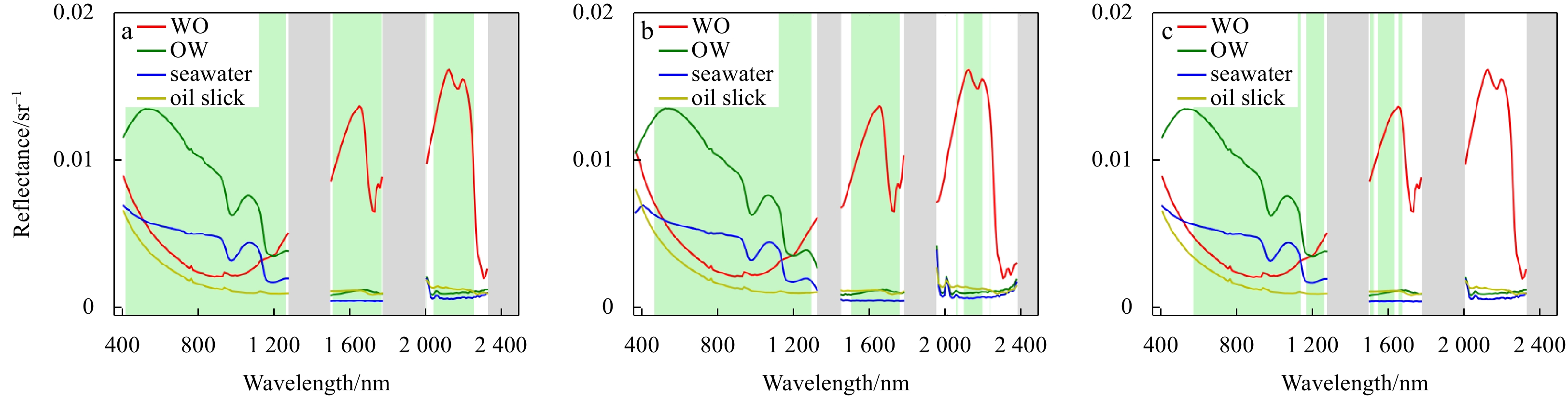
The reflectance data for the oil spill, its emulsions, and seawater are shown in Fig. 3a. WO has high reflectance in the 1200–2500 nm band with significant absorption features of the -C-H bonds at 1209 nm, 1725 nm, 1760 nm, 2310 nm and 2348 nm. OW has high reflectance in the 400–1300 nm band with light absorption of -O-H visible at 970 nm and 1160 nm. The absorption valley of crude oil -C-H in OW formed an absorption valley at 1210 nm, which is largely consistent with the experimental results of Lu et al. (2019). The spectral reflectance of crude oil is low because of its strong absorption of incident light and weak reflective and scattering properties. The spectral reflectance of seawater is also low because of the strong absorption of the water column; the reflectance peak at 1070 nm is due to the presence of a small amount of suspended material in the water. The presence of a reflectance peak at 1070 nm is caused by the absorption spectrum of the water column at 970 nm (Lu et al., 2008). Crude oil and seawater have a strong absorption of incident light, but the spectra of WO, OW, and crude oil in Fig. 3a show high reflectance and a decreasing trend in the visible range (400–800 nm), which is influenced by the strong Fresnel reflection of blue-violet light from the sky light on the oil-water surface and is unavoidable in outfield observation. However, in the airborne remote sensing data, this effect is removed by atmospheric correction; thus, the reflectance spectrum of the oil spill and its emulsions in the airborne remote sensing data show low reflectance in the visible range. In this study, we used the acquired ASD data for feature selection, mainly focusing on inter-band separability; thus, we did not consider the effect of Fresnel reflection differences in land-based and airborne data in subsequent experiments. This issue is discussed further in Section 4.

Figure  3.  Outfield land-based experimental oil spill hyperspectral data. a. Hyperspectral data acquired in the context of a Class Ⅰ water body. b. Hyperspectral data acquired in the context of a Class Ⅱ water body. The grey bars indicate the atmospheric absorption bands.

DownLoad: Full-Size Img PowerPoint

The trend of the spectral curve in Fig. 3b is basically consistent with that of Fig. 3a. The suspended material in seawater has an obvious scattering effect on the incident light, and thus the reflection spectrum of seawater shows reflection peaks at 560 nm and 700 nm. In addition, the reflection spectrum of OW is influenced by the background seawater, resulting in a spectrum that is very similar to that of the background seawater in the 450–950 nm band.

3. Models and methods

3.1 Oil emulsion identification model based on spatial-spectral feature fusion

Deep learning has shown significant advantages in processing high-dimensional data because of its evolving high-performance computing capabilities, and as a result there has been widespread interest in using deep learning for hyperspectral image target identification. Pixel-by-pixel classification of hyperspectral imagery using only spectral features may result in discrete points in the results that do not match the continuous distribution of the actual target, and thus the fusion of spectral and spatial features can effectively improve classification accuracy. We proposed a model for the identification of oil spill emulsions based on fused spatial and spectral features. This model can simultaneously use the two-dimensional geometric spatial information and one-dimensional spectral information of the target area to improve the identification accuracy and model generalization of oil spill emulsions. The model structure is shown in Fig. 4.

Figure  4.  Oil emulsion identification model based on the fusion of spatial and spectral features.

DownLoad: Full-Size Img PowerPoint

The model consists of two parts: feature selection and a three-dimensional convolutional neural network (3D-CNN). Hyperspectral remote sensing images have many image dimensions, and the number of bands of the two types of airborne hyperspectral data used in this study is 224 and 126, respectively. This could lead to dimensional explosion and the Hughes problem for deep learning models, and thus dimensionality reduction of hyperspectral images is necessary. The 3D-CNN uses 3D convolutional kernels to process the input data and is able to extract both spatial and spectral features of the image, which has significant advantages for the processing of hyperspectral remote sensing images.

3.2 Spectral feature selection based on the SD threshold and MI

Methods for hyperspectral remote sensing image dimensionality reduction consist of two main types: feature extraction and feature selection. Feature selection methods eliminate redundant bands and determine the optimal subset of features to reduce the number of features. Feature selection retains the physical characteristics of the original band and is widely used. Regarding target identification problems, feature selection methods can be mainly divided into two categories based on their algorithmic principles. The first category is to search all bands based on the criterion function to obtain a subset of bands that satisfy the optimal solution of the criterion function, such as the optimal index factor method, sequential forward selection algorithm, etc. For the airborne hyperspectral remote sensing data used in this study, the number of bands is relatively high, exceeding 100 in total. This will increase the computational complexity of the band search method, and it is easy to fall into the problem of local optimal solutions, making it difficult to obtain a subset of bands that performs the best globally. The second category calculates the inter-class separability between various bands or band combinations based on evaluation indicators, and selects bands or band combinations with greater inter-class separability as the subset of feature bands. Commonly used evaluation indicators include J-M distance, spectral angle, inter-mean standard deviation, information entropy, etc. The J-M distance and spectral angle are commonly used to evaluate the separability of band combinations. Inter-mean standard deviation can effectively calculate the separability of single bands. Information entropy reflects the richness of the information carried by the band combination. Therefore, a feature band selection method based on standard deviation threshold-mutual information was constructed in this study, which can further remove the redundant bands while retaining the bands with differentiability. Additionally, it offers a simple calculation process and is suitable for feature selection problems with a small number of categories and a large number of bands.

The SD threshold is a commonly used feature selection method that determines the separability of feature classes in a single band by calculating the statistical distance of the band. The SD threshold is calculated as

where λ is the wavelength; a and b are two types of targets; M_λa and M_λb are the mean values of the spectral reflectance of a and b, respectively; and S_λa and S_λb are the SDs of the spectral reflectance of a and b, respectively.

If the absolute value of the difference between the mean spectral reflectance values of the two types of targets is greater than the sum of the SDs, then these two targets are considered to have separability at that wavelength.

Although the SD threshold method is intuitive and simple, it ignores the correlation between bands, especially in the classification of hyperspectral data into multiple classes, and the selected results still include redundant bands. In this study, MI was introduced to quantitatively describe the overall distribution of the redundant spectral information and facilitate the further removal of redundant bands to obtain a subset of features.

In probability theory and information theory, MI is a measure of the statistical correlation between two random variables (Qin et al., 2015; Ross, 2014), which is non-negative. The MI between two random variables is calculated as

where X and Y are two random variables; $ {S}_{x} $ and $ {S}_{y} $ are value domains of X and Y, respectively; and p(x, y) = P(X = x, Y = y) is joint probability density.

For different categories of spectral reflectance data, the reflectance of each band and its corresponding category label were treated as two sets of random variables. By calculating the statistics between the variables, we obtained the MI value, which characterizes the degree of interdependence between features and category labels, i.e., the degree to which knowing the reflectance of a band reduces the uncertainty of the category labels. Larger values of MI indicate greater dependence of the band and category labels with respect to each other. The MI of each band after filtering by the SD threshold was calculated, and the band with the higher MI value was selected as the characteristic band for distinguishing crude oil, seawater, WO, and OW. The MI threshold used in this study was determined by comparing the results of several calculations, and the effect of different MI thresholds on the feature selection results is discussed in Section 4.

3.3 3D-CNN model

The SD threshold-MI feature band selection only extracts the spectral features. To make full use of the spatial information of hyperspectral remote sensing images for oil spill emulsion identification, we used a 3D-CNN to simultaneously extract the spectral features and spatial features of oil spill emulsions. Oil spills and emulsions are mostly distributed in strips on the sea surface, and when different types of oil spill emulsions are mixed with seawater, the oil slick, seawater, and oil spill emulsions tend to show more fragmented and discrete distribution characteristics. The spatial resolutions of the airborne hyperspectral data used in this paper are 7.6 m (AVIRIS) and 0.016 m (S185). For some oil spills and emulsions that are distributed in fragments, the smaller the size of the convolution kernel in the spatial dimension, the easier it is to extract spatial features. The convolutional layer is the core layer used to build the 3D-CNN. Considering the spatial distribution pattern of the oil spill and emulsions, it is reasonable to set the size of the convolutional kernel to 3 in the spatial dimension. A larger convolutional kernel in the spectral dimension will improve the global performance for spectral feature extraction, but it will increase the number of parameters and the computational effort of the model; a smaller convolutional kernel in the spectral dimension enables the network to be deeper, introducing more non-linearities and improving the identification performance of the model. In the method proposed in this paper, a convolution kernel of size 3 × 3 × 3 is specified. In Section 4, we discuss the effect of changing the size of the convolution kernel in the spectral dimension on the identification results. The features are extracted by the convolutional kernels, which traverses the spatial and spectral dimensions of the full input data to get the dot product, calculated as

where Z is the result of the convolution; p, q, and k are the number of rows, columns, and channels of the convolution kernel, respectively; w_i, v_i, and u_i are respectively the weights and pixel values of point I; b denotes the bias value.

The convolution outputs a feature cube that contains both spectral and spatial features. Then, we introduce a non-linear activation function to the convolution result for activation. The mainstream nonlinear activation functions include functions such as the rectified linear unit (ReLU) or sigmoid (Zhou et al., 2017). In the proposed method, we use ReLU as the activation function. ReLU has low computational complexity and faster convergence than other activation functions. Its formula is defined as

To reduce feature loss in the spatial and spectral dimensions of the data, a pooling layer was not added to the 3D-CNN model. After two convolutions, the data were fed into the fully connected layer and a softmax function was introduced to calculate the probability values of the input data corresponding to all the labels. The final output is the identification result.

4. Results and discussion

4.1 Analysis of oil emulsion identification results

4.1.1   Outfield airborne hyperspectral image identification results

The ASD data acquired in Section 2.2 for the Class Ⅱ water background were downsampled with respect to spectral resolution to obtain spectral reflectance data consistent with the S185 sensor band, as shown in Fig. 5. The SD threshold-MI method was used to select feature bands from the downsampled spectral data, resulting in 100 feature bands, as indicated by the green bands marked in Fig. 5. The characteristic bands are basically located at 450–850 nm and 850–950 nm. The reflectance spectrum of the four targets are relatively similar and not easily distinguishable.

Figure  5.  Hyperspectral data of oil spill emulsions in the context of a Class Ⅱ water body. The spectrum is downsampled to 126 bands, and the green bars are the selected feature band intervals.

DownLoad: Full-Size Img PowerPoint

The airborne hyperspectral imagery and simultaneous 4K imagery acquired as described in Section 2.1.1 were used to conduct the oil spill emulsion identification experiments. The distribution status of crude oil, WO, and OW in the pool were determined from the 4K images, as shown in Fig. 6a. The OW used in this experiment was diluted by seawater in the pool, and the distribution of OW could not be judged by visual interpretation. Moreover, because the background is a Class Ⅱ water body, the reflection spectra of OW are not easily distinguishable from those of the background water body. Therefore, OW in the enclosure grid is treated as seawater, and the identification targets are crude oil, WO, and seawater. The distribution areas of WO, seawater, and crude oil were delineated using visual interpretation, as shown in Fig. 6b, with 10% of the targets in each category selected as labels.

Figure  6.  S185 airborne hyperspectral remote sensing imagery. a. Simultaneous 4K image; b. visual interpretation result. The upper left, upper right, lower left and lower right enclosures are numbered No. 1, No. 2, No. 3, and No. 4, respectively. No. 1 was filled with crude oil, No. 2 was filled with WO at a volume concentration of 80%, No. 3 contained pure seawater, and No. 4 contained OW at a volume concentration of 0.1%.

DownLoad: Full-Size Img PowerPoint

The proposed oil emulsion identification model was trained using the labelled data. Note that the training and test sets were divided in a ratio of 2:8. The trained model was then used to identify oil spill emulsion in the global image, and the identification results are shown in Fig. 7a. The results show that the crude oil and seawater in enclosure No. 1 as well as the WO and seawater in enclosure No. 2 are well distinguished, with a few misclassifications of crude oil and WO. A small amount of crude oil and WO spilled from enclosures No. 1 and No. 2 into enclosures No. 3 and No. 4, all of which are effectively identified. The accuracy of the classification results was evaluated using the global visual interpretation results, as shown in Table 1, with an overall accuracy of 95.15% and a Kappa coefficient of 0.92.

Figure  7.  Results of airborne hyperspectral image identification for outfield experiments. a. Identification result. b. 4K image.

DownLoad: Full-Size Img PowerPoint

Table  1.  Accuracy evaluation of the airborne hyperspectral image identification results for the outfield experiments

Target	Precision	Recall	F1 score
WO	0.92	0.96	0.94
Seawater	0.93	0.94	0.93
Oil slick	0.97	0.95	0.96

 | Show Table

DownLoad: CSV

Compared with the synchronized acquisition of the 4K image in Fig. 7b, the model can make more accurate identification of crude oil, WO and seawater, preliminarily demonstrating the feasibility of using feature selection on hyperspectral data and utilizing its spatial and spectral characteristics for the identification of oil emulsions in simulated marine oil spill scenario. This experiment also shows that for the identification of oil emulsions, the influence of the background water body needs to be considered. The seawater used in this experiment is a Class Ⅱ water body. Due to the strong absorption of oil and WO in the visible-near infrared range (450–950 nm), the background water signal in the reflectance spectrum is low, which can clearly exhibit spectral differences between the oil/WO and the background water. As for OW, crude oil is distributed in the form of small droplets in the water. These oil droplets exhibit strong backscattering of incident light, causing OW to have a higher reflectance in the visible-near infrared band. Additionally, OW has a relative higher water content, making it more likely to display the signal of the background water in its reflectance spectrum. Consequently, OW exhibits similar reflectance spectrum to seawater. The background water bodies of oil spills occurring in offshore are mostly Class Ⅱ water bodies. Therefore, it may be challenging to differentiate between OW and seawater by using remote sensing data in the visible- near infrared band only. It is necessary to consider utilizing the spectral characteristics of OW in the shortwave infrared (SWIR) range for improved identification of OW and seawater.

4.1.2   AVIRIS hyperspectral image identification results

The ASD data acquired as described in Section 2.2 for a Class Ⅰ water background were downsampled with respect to spectral resolution to obtain spectral reflectance data consistent with the AVIRIS bands, leaving 160 bands after removal of the atmospheric absorption bands. The SD threshold-MI method was used to select features from the downsampled spectral data, resulting in 134 feature bands, as indicated by the green bands marked in Fig. 8. The selected characteristic bands are mainly concentrated in the ranges of 450–1300 nm, 1500–1780 nm, and 2050–2220 nm, which basically includes the absorption characteristics of the functional groups in oil emulsions, except for the bands with similar reflectance spectrum.

Figure  8.  Hyperspectral data of oil emulsions in the context of a Class Ⅰ water body. The spectrum is downsampled to 224 bands. The green bars are the selected feature band intervals and the grey bars are the atmospheric absorption bands.

DownLoad: Full-Size Img PowerPoint

Using study area 1 as the training area, the labels were set according to visual interpretation, as shown in Fig. 9a, where 50% of the labels were used for accuracy evaluation and were not involved in the training and testing of the model. The ratio of the training and test sets was 6:4. The trained oil emulsion identification model was used to identify oil emulsion on study area 1 imagery, and the results are shown in Fig. 9b. An accuracy evaluation was carried out on the identification results, as shown in Table 2, yielding an overall accuracy of 91.80% and a Kappa coefficient of 0.86.

Figure  9.  Study area 1 label distribution and identification results. a. Label distribution. The image is a false color composite: red: 1672 nm, green: 832 nm, blue: 658 nm. b. Identification results.

DownLoad: Full-Size Img PowerPoint

Table  2.  Accuracy evaluation of identification results for study area 1

Target	Precision	Recall	F1 score
WO	0.78	0.94	0.85
OW	0.83	0.82	0.82
Seawater	0.96	0.98	0.97
Oil slick	0.93	0.78	0.85

 | Show Table

DownLoad: CSV

On the data for study area 1, the model was able to achieve relatively accurate identification for WO, OW, oil slick and seawater. In particular, it was able to distinguish between different types of oil emulsions in areas with relatively discrete distributions of WO and OW, as well as mixed distributions of WO and OW. The distribution of emulsified oil and non-emulsified oil in the identification result image corresponds to actual oil spills scenarios. That is, WO and OW phases do not distribute independently; they are usually surrounded by some non-emulsified oil in the middle. These non-emulsified oil are closely associated with oil emulsions and have a higher brightness than the background seawater. Due to the influence of marine environmental dynamics, oil spills and its emulsions are generally distributed in long, thin strips on the sea surface.

The spectral reflectance of three sampled points in the WO, OW, oil slick, and seawater areas are shown in Fig. 10. The spectral responses of WO and OW in the near-infrared band are clearly characterized, whereas the spectral reflectance of oil slick is slightly higher than that of seawater. The selected characteristic band interval includes bands with significant spectral differences among four target types, indicating that in practical oil spill scenarios, the spatial and spectral information of airborne remote sensing images can be utilized for the identification of oil emulsions.

In addition to 3D-CNN, two-dimensional and one-dimensional convolutional neural networks (2D-CNN, 1D-CNN) are also widely applied in remote sensing image recognition and spectral classification. Machine learning algorithms have also shown good accuracy in the classification of hyperspectral images, for example, support vector machines (SVM). Based on the study area 1 data, we conducted comparative experiments to analyze the effectiveness of 1D-CNN, 2D-CNN and SVM in the identification of oil emulsions. The results and accuracy evaluation are shown in Fig. 11 and Table 3, respectively.

The results show that all three classifiers can identify oil emulsions with overall accuracy greater than 87% and Kappa coefficient of approximately 0.8, which are lower than those of 3D-CNN (overall accuracy: 91.80%; Kappa coefficient: 0.86). Furthermore, the precision and recall vary greatly across each category and the identification of WO and OW is poor for all three classifiers. According to the principle of convolutional neural networks, 2D-CNN focus on the spatial information of images, while 1D-CNN focus on the spectral information of images. Compared to the identification results of 3D-CNN(Fig. 9b), 2D-CNN and 1D-CNN showed poorer performance in identifying WO and OW with scattered patterns. There are also significant differences in distinguishing between oil slick and seawater. Figure 11c shows that SVM exhibits obvious misclassification for oil-slick and less effectively identified WO and OW emulsions. SVM is a linear machine learning algorithm and is not as good at extracting and representing data features as CNN through operations such as convolution and nonlinear mapping. The results above demonstrate that utilizing both spatial and spectral features can enhance the accuracy of identification for oil emulsions.

Figure  10.  Spectral reflectance of sampled pixels in study area 1. The grey bars are the atmospheric absorption bands.

DownLoad: Full-Size Img PowerPoint

Figure  11.  Identification results of different classifiers for study area 1. a. 2D-CNN classifier identification results. b. 1D-CNN classifier identification results. c. SVM classifier identification results.

DownLoad: Full-Size Img PowerPoint

Table  3.  Comparison of the overall accuracy (OA) of the identification results using different classifiers in study area 1

Classifier (OA and Kappa coefficient)	Target	Precision	Recall	F1 score
2D-CNN (OA = 87.02%, Kappa coefficient = 0.78)	WO	0.62	0.98	0.76
	OW	0.87	0.72	0.79
	seawater	0.90	0.99	0.94
	oil slick	0.97	0.64	0.77
1D-CNN (OA = 87.82%, Kappa coefficient = 0.82)	WO	0.46	0.98	0.63
	OW	0.91	0.78	0.84
	seawater	0.99	0.93	0.96
	oil slick	0.92	0.85	0.88
SVM (OA = 87.93%, Kappa coefficient = 0.78)	WO	0.72	0.99	0.83
	OW	0.87	0.92	0.89
	seawater	0.99	0.87	0.93
	oil slick	0.61	0.84	0.71

 | Show Table

DownLoad: CSV

4.2 Analysis of the spatial and temporal transferability of the oil emulsion identification model

Using study areas 2 and 3 as migration zones, the oil emulsion identification model trained in Section 4.1.2 was used for identification experiments, and the identification results are shown in Figs 12b and d. In study areas 2 and 3, labels were set on the basis of visual interpretation to evaluate the identification results. The accuracy evaluation results are shown in Tables 4 and 5. The results for study area 2 had an overall accuracy of 80.69% and a Kappa coefficient of 0.73; those for study area 3 had an overall accuracy of 86.53% and a Kappa coefficient of 0.80.

Figure  12.  Spatial and temporal migration identification results obtained by the oil emulsion identification model. a and c. Study areas 2 and 3, respectively, false-color composite: red: 1672 nm, green: 832 nm, blue: 658 nm. b and d. The model identification results of a and c, respectively. Study area 2 is a spatial migration area of study area 1 and study area 3 is a spatial–temporal migration area of study area 1.

DownLoad: Full-Size Img PowerPoint

Table  4.  Accuracy evaluation of the identification results for study area 2

Target	Precision	Recall	F1 score
WO	0.85	0.73	0.79
OW	0.8	0.99	0.88
Seawater	0.99	0.7	0.82
Oil slick	0.63	0.93	0.75

 | Show Table

DownLoad: CSV

Table  5.  Accuracy evaluation of the identification results for study area 3

Target	Precision	Recall	F1 score
WO	0.98	0.79	0.87
OW	0.72	0.98	0.83
Seawater	0.95	0.83	0.97
Oil slick	0.78	0.93	0.85

 | Show Table

DownLoad: CSV

Compared with the identification results in the training area, the accuracy of the identification results in the spatial-temporal migration areas of the model has decreased, but the overall identification results are effective. For areas with a mixed distribution of oil emulsions, the model can accurately distinguish between WO and OW. For oil slicks with a more discrete distribution and lower concentrations, the model is able to distinguish between them and seawater. The results show that the oil spill and emulsions can be identified under both spatial and spatial-temporal migration conditions, and the model constructed in this paper is stable.

The generalization ability of CNN models is usually closely related to the data set and model parameters. The more diverse the sample data in the training set is, the better the model performs in various scenarios. Therefore, in this study, when selecting sample data, we aimed to include as many samples with significant spectral differences within the same category as possible. Additionally, spectral standardization was applied to preprocess the data. Due to the potential discrepancies in the intensity of light between different images, the overall reflectance of the images may vary greatly. Spectral normalization can convert the spectral reflectance from different temporal and spatial conditions into a unified range, thereby improving the identification performance of the model across different images. In addition, regularization can also improve the generalization ability of the model. In this study, dropout was applied before the fully connected layer of the 3D-CNN model. The dropout rate was set to 0.3, which means that during the forward propagation, 30% of the activation values of the neural nodes were randomly set to zero. This setting can reduce the model’s reliance on certain local features, thereby further improve the generalization of the model.

4.3 Analysis of the spectral feature selection

To investigate the effect of spectral feature selection on the identification results, we used the study area 1 image without feature selection to conduct oil spill emulsion identification experiments, and the identification results are shown in Fig. 13a. The accuracy evaluation of the identification results is shown in Table 6. The overall accuracy was 89.18% and the Kappa coefficient was 0.82, which is a 2.62% reduction in overall accuracy and a 0.04 reduction in Kappa coefficient relative to the selected feature data. The F₁ scores for WO, OW, oil slick, and seawater are all reduced to varying degrees. In particular, there is a significant impact on the identification accuracy of OW. Comparing Fig. 13a with Fig. 13c of the selected-feature identification results, some of the WO is misclassified as OW and some of the seawater is identified as oil slick in the unselected-feature identification results.

Figure  13.  Comparison of the identification results with and without feature selection in study areas 1 and 3. a and b. Identification results obtained without feature selection for study areas 1 and 3, respectively. c and d. Identification results obtained with feature selection for study areas 1 and 3, respectively.

DownLoad: Full-Size Img PowerPoint

Table  6.  Accuracy evaluation of the identification results for study area 1

Target	No FS or FS	Precision	Recall	F1 score
WO	no FS	0.83	0.86	0.84
	FS	0.78	0.94	0.85
OW	no FS	0.55	0.82	0.66
	FS	0.83	0.82	0.82
Seawater	no FS	0.93	0.97	0.95
	FS	0.96	0.98	0.97
Oil slick	no FS	0.92	0.74	0.82
	FS	0.93	0.78	0.85
Note: Each type of target corresponds to two columns of accuracy evaluation results. The first column is the accuracy of the identification results without feature selection (no FS), and the second column is the accuracy of identification results with feature selection (FS).

 | Show Table

DownLoad: CSV

The model was used to conduct oil emulsion identification experiments on the study area 3 image without feature selection, and the identification results are shown in Fig. 13b. The accuracy evaluation of the identification results is shown in Table 7, yielding an overall accuracy of 83.08% and a Kappa coefficient of 0.75, a 3.45% reduction in overall accuracy and a 0.05 reduction in Kappa coefficient relative to the selected-feature data. WO and OW identification accuracies decrease substantially. Comparing the results in Fig. 13b with the results of feature selection in Fig. 13d, the identification results obtained with no feature selection show a significant number of misclassifications for WO and OW.

Table  7.  Accuracy evaluation of identification results for study area 3

Target	No FS or FS	Precision	Recall	F1 score
WO	no FS	0.99	0.61	0.75
	FS	0.98	0.79	0.87
OW	no FS	0.35	1.00	0.52
	FS	0.72	0.98	0.83
Seawater	no FS	0.95	0.85	0.90
	FS	0.95	0.83	0.97
Oil slick	no FS	0.82	0.93	0.87
	FS	0.78	0.93	0.85
Note: Each type of target corresponds to two columns of accuracy evaluation results. The first column is the accuracy of identification results without feature selection (no FS), and the second column is the accuracy of identification results with feature selection (FS).

 | Show Table

DownLoad: CSV

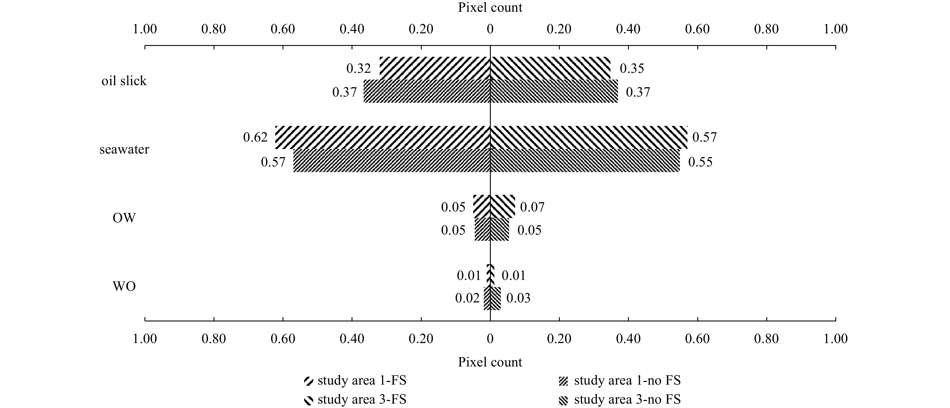
The proportion of WO, OW, seawater and oil slick pixels in each of the identification results in Fig. 13 were counted separately and the results are shown in Fig. 14. Relative to the identification results without feature selection, the proportion of seawater and OW pixels increased slightly, while the proportion of WO and oil slick pixels decreased in the identification results of study areas 1 and 3 when feature selection was used.

Figure  14.  Pixels statistics of the identification results obtained with feature selection (FS) and without feature selection (no FS) in study areas 1 and 3.

DownLoad: Full-Size Img PowerPoint

According to Fig. 13, for study area 1, the oil spill emulsion content is small and the spatial distribution is relatively discrete. After feature selection, some WO with small areas and mixed distribution with OW are more accurately identified, but the overall classification results do not change significantly.

For study area 3, the feature selection results were better than those without feature selection, specifically for the WO and OW mixed distribution area and the OW and oil slick mixed distribution area. The feature selection results more accurately identified WO and OW.

The experimental results indicate that performing feature selection on the data first can lead to a more accurate identification of oil spill and oil emulsions, and the model maintains good spatiotemporal transferability. This is because after feature band selection, the redundant bands in the hyperspectral data are removed, and only the spectral features that are effective for target identification are retained, which can reduce the computational complexity of the model. The feature selection process further simplifies and enhances the spectral features of the training set, avoiding overfitting and improving the generalization ability of the model.

4.4 Analysis of the sensor spectral resolution

Spectral feature selection reduces the spectral resolution of the data to some extent. To investigate the effect of spectral resolution on the proposed oil emulsion identification model, we downsampled the spectral resolution of the AVIRIS data. Simulated spectra with spectral intervals of 30 nm, 60 nm and 80 nm were each obtained using the ASD data described in Section 2.2, as shown in Fig. 15. The effects of the reduction in spectral resolution on seawater and oil slick spectra are minimal, thus only the effects on WO and OW spectra are analyzed in this paper. When the spectral resolution is 30 nm, the absorption features of the -C-H and -O-H bonds in WO and OW remain; when the spectral resolution is 60 nm, the absorption features of the -C-H bond in WO at 1725 nm and 1760 nm disappear; when the spectral resolution is 80 nm, the absorption features of the -C-H bond in WO at 2310 nm and 2348 nm disappear, and the absorption features of OW at 1160 nm are not obvious.

Figure  15.  AVIRIS spectrally downsampled data obtained from the ASD data. For the convenience of plotting, the reflectance data has been scaled as a whole and the y-axis does not display the reflectance values.

DownLoad: Full-Size Img PowerPoint

Using study area 1 as the training area and study area 3 as the migration area, the identification results at different spectral resolutions are compared in Fig. 16. The accuracy evaluation of the identification results are presented in Tables 8 and 9.

Figure  16.  Identification results at different spectral resolutions for study areas 1 and 3. a, b and c. Results of the identification of study area 1 at spectral resolutions of 30 nm, 60 nm and 80 nm, respectively. d, e and f. Results of the identification of study area 3 at spectral resolutions of 30 nm, 60 nm and 80 nm, respectively.

DownLoad: Full-Size Img PowerPoint

Table  8.  Comparison of the overall accuracy (OA) of the identification results at different spectral resolutions (SR) in study area 1

SR (OA and Kappa coefficient)	Target	Precision	Recall	F1 score
SR = 30 nm (OA = 90.46%, Kappa coefficient = 0.84)	WO	0.86	0.85	0.85
	OW	0.49	0.81	0.61
	seawater	0.94	0.98	0.96
	oil slick	0.94	0.93	0.93
SR = 60 nm (OA = 90.40%, Kappa coefficient = 0.83)	WO	0.8	0.85	0.82
	OW	0.51	0.79	0.62
	seawater	0.98	0.96	0.97
	oil slick	0.86	0.8	0.83
SR = 80 nm (OA = 89.41%, Kappa coefficient = 0.82)	WO	0.77	0.85	0.81
	OW	0.54	0.87	0.67
	seawater	0.94	0.99	0.96
	oil slick	0.95	0.71	0.81

 | Show Table

DownLoad: CSV

Table  9.  Comparison of the overall accuracy (OA) of the identification results at different spectral resolutions (SRs) in study area 3

SR (OA and Kappa coefficient)	Target	Precision	Recall	F1 score
SR = 30 nm, OA = 80.80%, Kappa = 0.72	WO	1.00	0.56	0.72
	OW	0.23	1.00	0.37
	seawater	0.95	0.84	0.89
	oil slick	0.79	0.93	0.85
SR = 60 nm, OA = 83.23%, Kappa = 0.76	WO	1.00	0.73	0.84
	OW	0.63	1.00	0.77
	seawater	0.97	0.78	0.86
	oil slick	0.69	0.95	0.80
SR = 80 nm, OA = 80.53%, Kappa = 0.72	WO	1.00	0.57	0.73
	OW	0.24	1.00	0.39
	seawater	0.90	0.87	0.88
	oil slick	0.84	0.88	0.86

 | Show Table

DownLoad: CSV

For study area 1, the overall accuracy and Kappa coefficient gradually decreased as the spectral resolution decreased, with the classification accuracy of the OW being significantly lower than the other three classes of targets. As shown in Figs 16a, b and c, misclassification occurs in regions where the WO and OW distributions are relatively discrete.

For study area 3, the overall accuracy and Kappa coefficient obtained at the reduced spectral resolution were lower than the results presented in Section 4.2, but the accuracy at a spectral resolution of 60 nm was higher than the accuracy at a spectral resolution of 30 nm, mainly due to the change in OW identification accuracy. When the spectral resolution was 60 nm, the F₁ scores for both seawater and oil slick in study area 3 decreased relative to the spectral resolution of 30 nm, the F₁ score for WO increased slightly, and the F₁ score for OW increased more significantly (by 0.54), thus improving the overall accuracy of the classification results relative to the spectral resolution of 30 nm. These results show that the effects of reduced spectral resolution on WO and OW identification are more pronounced after spatial and temporal migration.

It can be inferred that the reduced spectral resolution will affect the presentation of the spectral features of the oil emulsions, thus having a greater impact on the classification accuracy of the oil emulsions. There will be obvious misclassification phenomena in the identification of the mixed WO and OW distribution areas as well as some misclassification phenomena for the mixed oil slick and seawater distribution areas, which are not obvious. In addition, the decrease in spectral resolution has a significant impact on the model’s generalization ability. The variation in spectral resolution may lead to a substantial change in the classification accuracy of a certain category. In the study area 3, when the spectral resolution is 30 nm and 80 nm, the precision of OW is 0.23 and 0.24, respectively. However, when the spectral resolution is 60 nm, the precision of OW is 0.63, indicating that there is no strict proportional relationship between the model’s identification accuracy and the spectral resolution. It can be seen that the selection of bands is crucial for accurately identifying oil emulsions using deep learning models. On one hand, the sensor’s band settings need to be reasonable to exhibit the spectral characteristics of the oil emulsion. On the other hand, effective feature selection and identification algorithms need to be designed to minimize redundant information input and efficiently utilize the spatial-spectral characteristics of remote sensing data.

4.5 Parametric analysis of the proposed oil spill emulsion identification model

4.5.1   Differential analysis of land-based/airborne hyperspectral data

The ASD data obtained in this paper are affected by the strong Fresnel reflection of blue-violet light from sky light occurring on the oil-water surface. Crude oil and oil spill emulsions exhibit high and decreasing reflectance in the visible range (400–800 nm). The intensity of the Fresnel reflection is related to the observation geometry, and the Fresnel reflection of skylight cannot be avoided in land-based outfield experiments. In airborne remote sensing data, this effect is removed by atmospheric correction, and thus the reflectance spectrum of the oil spill and its emulsions in the airborne remote sensing data shows low reflectance in the visible range. In this paper, the acquired ASD data is used for feature selection, mainly focusing on inter-band separability, i.e., the degree to which targets can be distinguished in each band. Although the reflectance spectra of oil emulsions, crude oil, and seawater in land-based experiments are affected by the Fresnel reflection of skylight, the impact on the spectral reflectance difference between different targets is limited, and the band separability between different targets is not greatly affected by this. For land-based and airborne hyperspectral data, this difference in Fresnel reflection in the visible band has a limited effect on band separability. To retain the wavebands with strong separability between the oil spill and its emulsions as much as possible, the characteristic wavebands in the visible range of the feature selection results were retained in this study. The results show that when ignoring the Fresnel reflection difference between land-based and airborne hyperspectral data in the visible range, the proposed feature selection method still demonstrates advantages in airborne oil spill identification. The exact impact of this difference on the identification of oil spill emulsions and the methods to correct or remove this difference need to be further investigated in depth through experiments and analysis.

4.5.2   MI threshold selection analysis

The selection of the MI threshold affects the final feature band selection. To remove redundant bands while retaining as many of the spectral characteristics of the oil emulsion as possible, the MI threshold in the proposed method was determined by comparing the results of several calculations. Taking the selection of characteristic bands of the AVIRIS data as an example, the ASD data acquired as described in Section 2.2 for a Class Ⅰ water background were downsampled with respect to spectral resolution to obtain spectral reflectance data consistent with the AVIRIS bands, leaving 160 bands after removing the atmospheric absorption bands. The mean value of the MI was calculated as 0.83 for the data filtered by the SD threshold method. The MI thresholds were set to 0.6, 0.7, and 0.8 respectively, and the final characteristic band intervals were obtained as shown in Fig. 17. When the MI threshold is 0.6, the number of filtered characteristic bands is 148, which still includes many redundant bands. When the MI threshold is 0.7, the number of filtered characteristic bands is 134; more bands are removed, but the functional group absorption characteristic bands of oil emulsions are basically retained. When the MI threshold is 0.8, the results yield 92 characteristic bands which do not include 2000–2400 nm. As a result, the functional group absorption characteristics of WO in this range cannot be demonstrated in the characteristic bands. This comparison reveals that it is reasonable to set the mutual MI at 0.7.

Figure  17.  Feature selection results for different MI thresholds. a, b and c. Results of feature band selection for MI thresholds of 0.6, 0.7 and 0.8, respectively. The green bars are the selected feature band intervals and the grey bars are the atmospheric absorption bands.

DownLoad: Full-Size Img PowerPoint

4.5.3   3D-CNN convolutional kernel size analysis

To investigate the effect of the size of the convolutional kernel in the spectral dimension on the model, we changed the size of the convolutional kernel of the 3D-CNN to 5 × 3 × 3 and 7 × 3 × 3, respectively, while the other parameters remained unchanged. The model was trained using the study area 1 image and experiments were carried out on the identification of oil emulsions using the trained model for study areas 2 and 3, the results of which are shown in Fig. 18.

Figure  18.  Model identification results for different convolutional kernel sizes. a, b and c. Identification results for study areas 1, 2 and 3, respectively, when the convolution kernel is 5 × 3 × 3. d, e and f. Identification results for study areas 1, 2 and 3, respectively, when the convolution kernel is 7 × 3 × 3.

DownLoad: Full-Size Img PowerPoint

By varying the size of the convolution kernel, the model is able to effectively distinguish different types of oil spill emulsions and maintain a relatively high accuracy after spatial and temporal migration. For the identification of oil slicks, the results vary slightly with respect to convolution kernel size. The identification results for convolutional kernels of 5 × 3 × 3 and 7 × 3 × 3 did not change significantly compared with the recognition results for convolutional kernels of size 3 × 3 × 3. However, when the convolutional kernel size was 7 × 3 × 3, a more obvious misclassification of some WO as OW appeared in the identification results of study area 3. These results reveal that the size of the convolutional kernel has a limited effect on the identification accuracy of the model, and that a smaller convolutional kernel is relatively more effective.

5. Conclusions

Hyperspectral remote sensing is an important tool for the accurate identification of different types of marine oil emulsions. In this paper, a model for the identification of oil emulsions by fusion of spatial-spectral features was established. We obtained the characteristic bands that can distinguish between crude oil, WO, OW, and seawater, and conducted identification experiments on oil emulsions against different background water and under various spatial-temporal conditions. Several conclusions can be derived as follows. (1) The SD threshold-MI feature selection method is able to effectively extract feature bands that can distinguish WO, OW, oil slick, and seawater. The number of bands was reduced from 224 to 134 after feature selection on the AVIRIS data and from 126 to 100 on the S185 data. (2) With feature selection, the overall accuracy and Kappa coefficient of the identification results for the training area are 91.80% and 0.86, respectively, improved by 2.62% and 0.04, and the overall accuracy and Kappa coefficient of the identification results for the migration area are 86.53% and 0.80, respectively, improved by 3.45% and 0.05. Especially for the identification of WO and OW mixed distribution areas and oil slick and seawater mixed distribution areas, the results are more accurate with feature selection. (3) The oil emulsion identification model has a certain degree of transferability and can effectively identify oil spill emulsions for AVIRIS data collected at different times and locations, with an overall accuracy of more than 80%. (4) The spectral resolution influences the identification accuracy of the model. As the spectral resolution decreases, the model will show different degrees of misclassification for the mixed distribution areas of oil slick and seawater as well as the mixed distribution areas of WO and OW.

When marine oil spills occur, there are still many difficulties in obtaining field measurement data such as oil spill volume, oil spill emulsion distribution, and oil spill emulsion concentration. The lack of field measurement data limits the accuracy evaluation of the identification results. In addition, the identification of marine oil spill emulsions is influenced by other factors such as environmental conditions at the sea surface and sun glint. However, the model developed in this paper does not take into account the effect of sun glint on the spectrum of oil spill emulsions. Further research is required to develop models that are suitable for different sun glint conditions.