Antarctic sea ice is an important part of the Earth’s atmospheric system, and satellite remote sensing is an important technology for observing Antarctic sea ice. Whether Chinese Haiyang-2B (HY-2B) satellite altimeter data could be used to estimate sea ice freeboard and provide alternative Antarctic sea ice thickness information with a high precision and long time series, as other radar altimetry satellites can, needs further investigation. This paper proposed an algorithm to discriminate leads and then retrieve sea ice freeboard and thickness from HY-2B radar altimeter data. We first collected the Moderate-resolution Imaging Spectroradiometer ice surface temperature (IST) product from the National Aeronautics and Space Administration to extract leads from the Antarctic waters and verified their accuracy through Sentinel-1 Synthetic Aperture Radar images. Second, a surface classification decision tree was generated for HY-2B satellite altimeter measurements of the Antarctic waters to extract leads and calculate local sea surface heights. We then estimated the Antarctic sea ice freeboard and thickness based on local sea surface heights and the static equilibrium equation. Finally, the retrieved HY-2B Antarctic sea ice thickness was compared with the CryoSat-2 sea ice thickness and the Antarctic Sea Ice Processes and Climate (ASPeCt) ship-based observed sea ice thickness. The results indicate that our classification decision tree constructed for HY-2B satellite altimeter measurements was reasonable, and the root mean square error of the obtained sea ice thickness compared to the ship measurements was 0.62 m. The proposed sea ice thickness algorithm for the HY-2B radar satellite fills a gap in this application domain for the HY-series satellites and can be a complement to existing Antarctic sea ice thickness products; this algorithm could provide long-time-series and large-scale sea ice thickness data that contribute to research on global climate change.
Antarctic sea ice significantly influences the global climate and environment in the Earth system by reflecting the incoming solar radiation between the oceans and atmosphere (Holland et al., 2006; Turner et al., 2009; Crosta et al., 2022). The sea ice freeboard and thickness are important parameters of the cryosphere affecting the heat flux and are also indicators of global climate change (Comiso et al., 2008; Tian et al., 2020). Several approaches to observing the sea ice freeboard and thickness have been proven to be applicable, and they each have individual advantages and disadvantages (Haas et al., 2009; Williams et al., 2015). In-situ and ship-based measurements can provide the most accurate sea ice information, while the spatial and temporal distributions of such data are limited (Worby et al., 2011; Ozsoy-Cicek et al., 2013). In contrast, satellite altimetry has been demonstrated to be an effective way to obtain large-scale and long-time-series sea ice freeboard and thickness data in Antarctica (Zwally et al., 2008; Kwok, 2010; Wang et al., 2022). With the continuous launch and renewal of satellite altimetry, more algorithms for the retrieval of Antarctic sea ice freeboard and thickness have been developed (Wang et al., 2013; Markus et al., 2017; Kwok et al., 2020).
Satellite altimetry sensors can be divided into lidar and radar instruments according to the different onboard sensors (Farrell et al., 2011; Weissling et al., 2011). Laxon et al. (2003) proposed the first examination of the Arctic sea ice thickness distribution using European Remote Sensing Satellites (ERS-1/2) radar altimeter data followed by Envisat mission data. Since April 2010, CryoSat-2, a mission of the European Space Agency (ESA), has provided radar altimeter data that can be used to obtain the surface elevation of Antarctica, though the latitudinal limit is 88°S (Fons et al., 2021). The CryoSat-2 mission, measuring the surface elevation of sea ice, could be employed to estimate the sea ice freeboard, which can then be converted into the sea ice thickness (Laxon et al., 2013). According to the characteristics of CryoSat-2 altimeter data, new algorithms for estimating the sea ice freeboard and thickness are consistently proposed and summarized (Kurtz et al., 2014; Helm et al., 2014; Ricker et al., 2014). The retracking algorithm proposed by Helm et al. (2014) is now a commonly used algorithms for estimating the sea ice freeboard. The Chinese Haiyang-2 (HY-2) satellite, launched on August 16, 2011, carried four kinds of microwave instruments for observing dynamic ocean, atmosphere, and ice environment parameters at the global scale (Chen et al., 2021; Jia et al., 2020). The radar altimeter, as part of the HY-2 mission, operates at 13.59 GHz (Ku-band) and 5.25 GHz (C-band) and can provide along-track sea surface heights (SSH) and waveform information that can be used to estimate the sea ice freeboard and thickness in Antarctica (Landy et al., 2020).
The HY-2 satellite set the foundation for long-term ocean monitoring in Antarctica and eventually improved our understanding of the significance of the Antarctic waters in the global climate system (Zhang et al., 2021). HY-2 satellite data are divided into Interim Geophysical Data Records (IGDR), Sensor Geophysical Data Records (SGDR), and Geophysical Data Records (GDR) depending on the processing steps. The waveform information and surface elevation data are stored in the SGDR and GDR products, which are available for estimations of the sea surface height using previously developed algorithms, especially for CryoSat-2 (Lee et al., 2016). CryoSat-2 waveform parameters such as purse peakiness (PP), leading edge width (LEW), stack standard deviation (SSD), maximum power (MAX) and sigma0 can be used to classify sea ice and lead (Armitage and Davidson, 2014). Similar to other radar altimeter data, HY-2 can distinguish between sea ice and lead using waveform information because different ground objects have different waveforms. Subsequently, the sea surface heights can be confirmed by the lead classification, and the sea ice freeboard and thickness can be converted (Yi et al., 2011). Considering the difference between the HY-2 sensor and other radar satellite altimeters, the original algorithm needs further refinement, especially in terms of the selection and setting of retrieval parameters (Zhong et al., 2023). Currently, the commonly used algorithms for applying HY-2 satellite data in polar regions involve obtaining sea ice and lead information from single-waveform features, while HY-2B data have never been used to confirm Antarctic sea surface heights to estimate the Antarctic sea ice freeboard or thickness (Jiang et al., 2019).
There are three objectives in this study: (1) to build a dataset of lead in Antarctica and generate a decision tree for classifying sea ice and lead from the Antarctic lead dataset, (2) to calculate the sea surface heights from the classification information and estimate the Antarctic sea ice freeboard and thickness from HY-2 satellite altimeter data, and (3) to compare the HY-2-derived sea ice thickness with other sea ice thickness products and evaluate the accuracy of the HY-2B-derived sea ice thickness. In the remainder of this paper, we first introduce the data and methods in Section 2. Then, we present and analyze the lead extraction and sea ice thickness retrieval results in Section 3. Section 4 focuses on a discussion of the results. Finally, the conclusions drawn in this paper are summarized in Section 5. The study area considered herein is the whole Antarctic waters existing sea ice, which includes five sectors: the Weddell Sea, the Bellingshausen and Amundsen Seas, the Ross Sea, the Pacific Ocean, and the Indian Ocean (Fig. 1). We analyze and discuss the results from the perspective of the whole Antarctic waters as well as these five individual sea sectors.
Figure
1.
Five sea areas of the Antarctic waters, with an overlaid background of the maximum (blue, September 20, 2019) Antarctic sea ice extent in 2019. The whole Antarctic waters refers to the sea areas around the Antarctic continent within latitudes above 60°S.
The HY-2B satellite is the second generation of the HY-2 mission launched by China on November 24, 2018 to sustainably monitor dynamic ocean environments. The altitude of the HY-2B satellite is approximately 971 km, and the observation range of the satellite spans from 80.7°N to 80.7°S, encompassing the whole Antarctic waters (Jia et al., 2020). The HY-2B altimeter data product provides multiple levels of data according to the degree of data processing. In this study, we used the HY-2B level-2 GDR and SGDR data to acquire surface elevation and 128-bin waveform information at each measuring point from January 1, 2019 to December 31, 2019 to confirm the sea level heights and estimate the Antarctic sea ice freeboard and thickness. Table 1 shows the HY-2B parameters we used in this paper. The HY-2B data were downloaded from the data distribution system of the National Satellite Ocean Application Service (https://osdds.nsoas.org.cn/). It should be noted that the HY-2B data include the 20-Hz and 1-Hz parameters, and some of these parameters, such as the dry troposphere correction and wet troposphere correction, have only 1-Hz data. Interpolation was applied as an effective method to solve the differences between the 1-Hz data and 20-Hz data. We selected data from HY-2B throughout the Antarctic waters in 2019 for our experiment, where 2019 was the first full year after the launch of HY-2B.
Table
1.
Parameters of the HY-2B radar satellite data used in this study
Parameter name
Source
Application
Waveform_20hz_ku
SGDR products
retracking, generating a discrimination decision tree
The Aqua satellite was launched on May 18, 2012 and carried the Advanced Microwave Scanning Radiometer 2 (AMSR2) sensor. The AMSR2 provides accurate measurements of sea ice microwave emissions (brightness temperature) within the frequency range of 6.925 GHz to 89 GHz. These measurements have been employed to estimate the sea ice concentration and snow depth on sea ice. The AMSR2 snow depth has the advantage of a daily temporal coverage and a spatial coverage comprising the entire polar region; this dataset is thus an important source for Antarctic snow depth products (Lee et al., 2015).
In this study, the AMSR2 snow depth product compiled at the corresponding time as the HY-2B altimeter data was acquired from the U.S. National Snow and Ice Data Center (NSIDC) at https://nsidc.org/data/AU_SI12/versions/1. The NSIDC produces a unified Level-3 snow depth product with a spatial resolution of 12.5 km by applying the snow depth retrieval model proposed by Markus and Cavalieri (1998). The snow depth product was used as the input data for the sea ice thickness retrieval from the sea ice freeboard estimated by HY-2B based on the static equilibrium equation (Kurtz et al., 2009; Kern et al., 2015).
2.1.3
MODIS MYD29 ice surface temperature (IST)
Moderate-resolution Imaging Spectroradiometer (MODIS) is an instrument onboard the two polar observation satellites Terra (launched in 2000) and Aqua (launched in 2002), part of the National Aeronautics and Space Administration’s Earth Observing System (NASA-EOS). MODIS views the whole Antarctic waters every day and provides continuous measurements stored in 5-min tiles with a 1-km spatial resolution at nadir within an array containing 951 (along-swath) × 951 (across-swath) grid points (Drüe and Heinemann, 2004; Reiser et al., 2020). The MODIS MYD29 product provides ice surface temperatures in the Antarctic waters, including land and cloud masks, at a geometric resolution of 1 km. In this study, we used approximately 4000 IST grids covering the southern region of 55°S from the NSIDC (https://nsidc.org/data/myd29p1d/versions/6) to construct a dataset of lead throughout the Antarctic waters through an approach incorporating several existing lead detection algorithms (Willmes and Heinemann, 2015; Lee et al., 2016; Reiser et al., 2020). Common MODIS leads algorithms achieve over 90% identification of sea ice and 60% to 100% identification of leads based on visual interpretation validation dataset while MODIS images have better spatial coverage than Synthetic Aperture Radar (SAR) images with excellent ability to identify sea ice leads (Willmes and Heinemann, 2015). The IST dataset was then used to match the HY-2B altimetry point data from the same day and construct the HY-2B lead classification decision trees. This method of data matching may be subject to errors due to the method of sea ice drift, which is one of the directions of subsequent research.
2.1.4
Sentinel-1 SAR Images
Sentinel-1 is composed of two polar-orbiting satellites carrying C-band SAR sensors. Sentinel-1 SAR images have spatial resolutions of 10 m (interferometric wide, IW) and 40 m (extended wide, EW) and a relatively high image acquisition frequency for Antarctica due to the Sentinel-1 polar orbit characteristics (Landy et al., 2019). SAR images exhibit a great resolution to identify leads from Antarctic sea ice and monitor sea ice movement (Shi et al., 2014; Li et al., 2021). In this study, we selected Sentinel-1 SAR images with a short time interval with MODIS IST data to verify the accuracy of the MODIS-extracted leads. The Sentinel-1 IW-mode images are available closer to the coast and have much better resolution than the EW-mode images. However, IW-mode images are unable to cover as much area as EW mode images while ensuring the quantity and extent of the images. Finally, we selected eight Sentinel-1 SAR EW-mode images acquired from https://search.asf.alaska.edu/ after screening.
2.1.5
CryoSat-2 and ICESat-2 sea ice freeboard and ship-based observed sea ice thickness dataset
CryoSat-2 and Ice, Cloud and land Elevation Satellite-2 (ICESat-2) were launched in 2011 and 2018, respectively, providing high-precision radar and laser altimeter data (Kwok and Kacimi, 2018; Kwok et al., 2019). Currently, CryoSat-2 and ICESat-2 altimeter data play important roles in sea ice research. We downloaded CryoSat-2 L2 data from ftp://science-pds.cryosat.esa.int/ and ICESat-2 ATL10 data from https://nsidc.org/data/ATL10/versions/4 and then processed these data into monthly sea ice freeboard grids. Considering that CryoSat-2 and HY-2B altimetry are both radar satellite instruments, we chose the CryoSat-2 sea ice freeboard for comparison with the HY-2B-derived freeboard. Since lasers sense the elevation of the air-snow surface while radars sense the elevation of the snow-ice surface, we used ICESat-2 laser total freeboard to investigate the penetration of radar to snow combined with the HY-2B freeboard. We validated the HY-2B-derived sea ice thickness using ship-based observed sea ice thickness data from February 22 to March 29 in 2019 in Weddell Sea, published at https://doi.pangaea.de/10.1594/PANGAEA.901263.
2.2
Methods
2.2.1
Sea ice lead identification algorithm in the Antarctic from MODIS IST product
When MODIS is used to observe Antarctic sea ice, negative brightness is found mainly in areas with open water and leads (Willmes and Heinemann, 2015) (Fig. 2). Moreover, leads composed of thin ice and open water exhibit superior surface temperatures compared to Antarctic sea ice because the temperature of sea ice is well below the freezing point of sea water, as indicated by Arrow 1 in Fig. 2. Considering that leads are applied mainly to the classification of HY-2B altimeter measuring points in this study, we established the following requirements for the retrieved leads from the MODIS IST product: (1) the Antarctic MODIS IST product must be obtained on the same day as the HY-2B altimeter data, and the time period must cover as many days as possible; (2) the MODIS IST product must covers as much of the Antarctic waters as possible; and (3) the selection of leads must be based mainly on accuracy compared to quantity to ensure the correctness of the subsequent operations.
Figure
2.
MODIS-derived ice surface temperature on September 29, 2019, with a cloud mask (yellow) and Antarctic continent (gray). Arrow 1 refers to the area with a lead, and Arrow 2 represents an area of invalid values (cloud).
Based on the premise above, we selected MOIDS IST products for the whole Antarctic waters to extract leads from sea ice. A series of threshold determination methods, such as standard deviations, Otsu’s threshold and maximum entropy (Drüe and Heinemann, 2004; Reiser et al., 2020), were tested. These threshold methods are based on the surface temperature discrepancy between leads and sea ice and involve the separation of the temperature histogram in a certain range. We further employed the potential open-water (POTOWA) method to achieve the separation of sea ice and leads in the Antarctic waters for each image pixel (Drüe and Heinemann, 2004). When the POTOWA algorithm was applied, the MODIS IST data granule was segmented into 31 × 31-pixel cells or 51 × 51-pixel cells and then divided into 9 subcells to estimate a bilinear function according to the coordinate of the center of each subcell. The background temperature of each subcell was also estimated, and then POTOWA could be calculated. Theoretically, leads have higher values than surrounding pixels, especially for thick sea ice. Finally, we classified the leads using twice the standard deviation.
We compared and integrated all MODIS-extracted leads and fused them into a complete dataset by taking the intersection. Finally, Canny arithmetic was applied to detect the gradient and indicate the lead edge, which was integrated with the above products to form the final MODIS-extracted leads. This method described above effectively avoids the influence of clouds in images and ensures the veracity of the lead classification results. To assess the lead discrimination accuracy, we extracted sea ice leads from collocated Sentinel-1 images with corresponding time and location data through supervision classification combined with visual interpretation. The MODIS-extracted leads form a diurnal-scale dataset for sampling and validation.
2.2.2
Sea ice freeboard and thickness retrieval algorithm from HY-2B altimeter data
The first step in the retrieval of sea ice thickness from altimeter data is the estimation of the local sea surface reference (Xie et al., 2011); this requires the discrimination of sea ice and leads according to the measured surface elevation above a reference ellipsoid. The characteristics of HY-2B radar echo signals are an important basis for identifying sea ice and leads when measuring ocean and ice surfaces. When the echo is dominated by specular reflections, it means that the radar pulse is reflected from a smooth surface such as a lead. In this case, the bin window of power has a peak structure with a rapid rise and fall in power. In contrast, diffuse echoes occur while the HY-2B radar pulse is reflected from a rough surface, mainly including open water and ice floes in the Antarctic waters, in which case the power in the waveform window rises rapidly and decreases slowly. In this study, the parameters of a 128-bin waveform window, which represent the waveform characteristics of the window, were used to identify specular and diffuse echoes so sea ice and lead discrimination could be implemented. As important parameters, pulse peakiness and stack standard deviation have been frequently used for the determination of the echo type in previous sea ice freeboard retrievals involving the CryoSat-2 satellite radar altimeter (Armitage and Davidson, 2014), and the calculation of PP is as follows:
where PP is pulse peakiness, P is the power received over the waveform,and i is the i-th range bin of the whole waveform.
In addition, parameters such as the leading edge width (LEW), backscattering coefficient, maximum power, skewness, and kurtosis have been used to describe the characteristics of a waveform in a range window. In this study, we selected the PP, LEW, SSD, kurtosis, and maximum of the HY-2B SDR altimeter data by comparing the correlation between each waveform parameter and the MODIS lead classification to explore the criteria for sea ice and lead discrimination. Considering that partial noise exists in the HY-2B waveform, we performed Gaussian fitting to the HY-2B waveform data, which also plays an important role during waveform retracking for the HY-2B altimeter data.
To establish reasonable rules for sea ice and lead classification from HY-2B altimeter data, we applied classification and regression tree (CART) analysis (Lewis, 2000) to discriminate leads based on multiple waveform parameters. The basic principle of CART is to analyze the attributes of the sample, set the classification rules, subdivide the dataset down, and form a binary tree decision tree structure. A specific threshold value was set when making lead classification rules in the CART decision tree in this study. As the attribute value of the dataset reaches the threshold range, a branch node is generated; otherwise, the attributes of many datasets are rearranged and grouped until their attribute values falls within the threshold range. The CART algorithm has many functions and advantages of setting thresholds automatically, including strong practicability, high classification accuracy, powerful function and simple operation. We conducted the following steps in this paper. (1) Constructing the binary decision tree recursively using waveform parameters based on the training dataset-MODIS-extracted leads. (2) Pruning the generated binary decision tree and selecting the optimal subtree with the minimum loss function as the pruning criterion; in addition, the Gini coefficient was used to measure the loss in the pruning process of the CART classification decision tree. Finally, we ensured that the branches of the decision tree were sufficiently concise.
After estimating the local sea surface reference, we calculated the 10-km-averaged height ($ {h}_{\mathrm{m}} $) from the surface height ($ {h}_{\mathrm{o}\mathrm{b}\mathrm{s}} $) and then obtained the relative elevation by computing the difference between $ {h}_{\mathrm{o}\mathrm{b}\mathrm{s}} $ and $ {h}_{\mathrm{m}} $ (Spreen et al., 2006). We simply filtered the surface height data by the threshold method to remove some outliers. The sea ice freeboard was calculated as the difference between the relative elevation and sea surface reference, as shown in Eqs (2) and (3):
where $ {h}_{\mathrm{r}} $ is the relative elevation, $ {h}_{\mathrm{f}\mathrm{i}} $ is the sea ice freeboard and ${h}_{\mathrm{ssh}}$is the sea surface reference height (Fig. 3).
Figure
3.
Geometric relationships among the sea ice freeboard ($ {h}_{\mathrm{i}} $), snow depth (${h}_{\mathrm{s}}$) and sea ice thickness ($ {h}_{\mathrm{i}} $) measured by the HY-2B radar satellite altimeter.
The sea ice thickness can be calculated from the sea ice freeboard according to the static equilibrium equation (Kurtz and Markus, 2012; Kurtz et al., 2014). HY-2B is a radar altimeter that indicates that the sea ice heights provided by HY-2B GDR and SDR data do not include the snow depth over sea ice. We estimated the sea ice thickness ($ {h}_{\mathrm{i}} $) through Eq. (4) with the input of the sea ice freeboard ($ {h}_{\mathrm{fi}} $), snow depth ($ {h}_{\mathrm{s}} $), snow density ($ {{\rho }}_{\mathrm{s}} $), water density ($ {{\rho }}_{\mathrm{w}} $), and sea ice density ($ {{\rho }}_{\mathrm{i}} $). In this study, $ {{\rho }}_{\mathrm{s}} $ = 300 kg/m3, $ {{\rho }}_{\mathrm{w}} $ = 1023.9 kg/m3, and $ {{\rho }}_{\mathrm{i}} $ = 915.1 kg/m3 (Zwally et al., 2008), and the AMSR2-derived snow depth were used to calculate the Antarctic sea ice thickness.
3.1
MODIS-derived lead and HY-2B lead discrimination decision tree
We employed MODIS IST products to build the lead dataset through the method described in Section 2.2.1 and attempted to use these data as the sample set and the validation set. Figure 4 shows the comparison between the MODIS ice surface temperature and MODIS-derived leads. The extracted lead was located in an area with a relatively high brightness temperature compared to the surrounding area, consistent with the physical properties of lead in the Antarctic waters (Willmes and Heinemann, 2015). There were also some undetected clouds in the image that were patchy and reflected positive temperature anomalies, which our algorithm excluded. Notably, the edges of the extracted lead were fairly rough, and it was difficult to obtain complete morphological and size information as a result of the relatively low spatial resolution of the MODIS IST product. Moreover, we found that MODIS-derived leads were capable of covering the whole Antarctic waters every day, although many image areas were not available due to cloud cover.
Figure
4.
Comparison between the ice surface temperature and extracted leads on October 3, 2019: a. MODIS-derived ice surface temperature with cloud mask (yellow) and b. MODIS-derived leads with cloud mask (yellow).
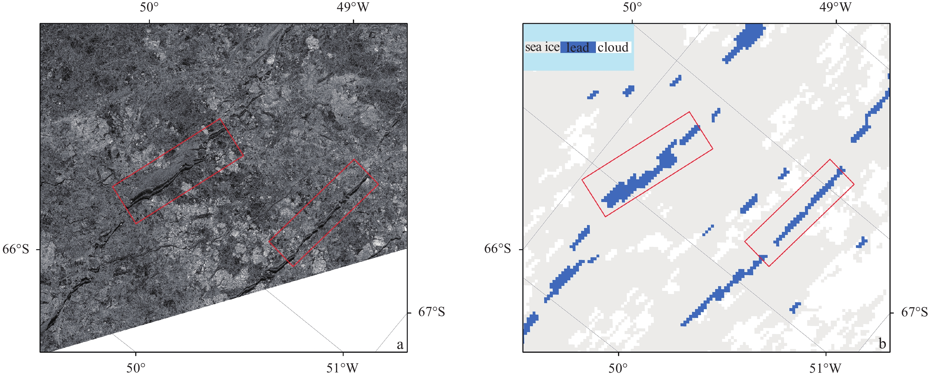
Subsequently, we validated the MODIS-derived leads using eight Sentinel-1 SAR images and the results of the validation are shown in the Table 2. The accuracy of MODIS sea ice leads was distributed between 0.6667 and 0.9576, with an overall accuracy of 0.8186. We found that the MODIS IST data were able to identify leads with large lengths and widths with relatively simple morphological features, especially in the area of the red rectangle in Fig. 5, and some refreezing leads could also be identified because the pixel values brighten up if the leads are refreezing or covered by frost flowers (Passaro et al., 2018). In addition, the relatively fine and short leads were difficult to distinguish due to the insufficient resolution, and the lead size obtained by MODIS IST data were also subject to deviations comparing with Sentinel-1 SAR images due to the limitations of the resolution, which was one of the issues we would be addressing in the future.
Table
2.
MODIS sea ice leads validation results based on Sentinel-1 SAR images
Figure
5.
Example of Sentinel-1 SAR images and corresponding MODIS-extracted leads on October 6, 2019: a. Sentinel-1 SAR images and b. MODIS-extracted leads.
Based on the existing MODIS-derived lead dataset, we applied the Cart tree method to generate a decision tree on the basis of the waveform information from the HY-2B radar satellite data. After several sample-set selections, training, and decision-tree pruning, we finally performed manual pruning of the decision tree (Fig. 6). In the pruning process, parameters such as the backscattering coefficient, left pulse peakiness and right pulse peakiness were removed. We ended up using 5 parameters to construct the decision tree, including the pulse peakiness, maximum value, kurtosis, leading edge width, and standard deviation. In this decision tree, pulse peakiness was the most important parameter because it reflected the waveform characteristics. We randomly selected two months of MODIS sea ice leads datasets (August and October) and built the datasets based on four approaches: (1) August as the sample set and October as the test set; (2) October as the sample set and August as the test set; (3) 70% of all data as the sample set and 30% of data as the test set; (4) 80% of all data as the sample set and 20% of data as the test set. Table 3 shows our testing of the lead and sea ice classification results with four groups of different sample sets and validation sets, indicating that we have achieved a classification accuracy exceeding 70%, while most areas have accuracies above 80%. To date, the pulse peakiness and leading edge width have often been used in classifications of CryoSat-2 radar data for lead discrimination. In contrast, our proposed decision tree expanded this analysis with other parameters (Fig. 6).
Figure
6.
HY-2B surface classification decision tree in Antarctica.
3.2
Antarctic sea ice thickness retrieved from HY-2B radar altimeter data
Based on the lead discrimination decision tree, we obtained the classification information of the measurement points for each HY-2B track and estimated the sea ice freeboard at each measurement point combined with the retracking elevation values. Then, the sea ice thickness grids were calculated through Eqs (2)–(4). Figure 7 shows the spatial distribution and temporal variation of Antarctic HY-2B monthly sea ice thickness in 2019. Relatively thick sea ice was concentrated mainly in the Weddell Sea throughout the whole year, and the coastal areas had thicker sea ice than the offshore areas in both the Antarctic summer and winter. The change in Antarctic sea ice from summer to winter is mainly reflected in the extent of sea ice, with large amounts of thinner sea ice appearing at the sea ice edge. The month with the smallest Antarctic sea ice extent in the year was February, and the month with the largest sea ice extent was October; this was not directly related to the magnitude of average sea ice thickness. The higher average Antarctic sea ice thickness from January to April may be due to the fact that the thinner sea ice in the marginal areas of the Antarctic has melted during this period, with a thicker layer of multi-year ice in the remaining sea ice, which skews the overall results. The large uncertainty in the HY-2B data could also lead to an overestimation of sea ice thickness in some areas. Generally, the HY-2B radar satellite has a good ability to retrieve the monthly average Antarctic sea ice thickness. HY-2B satellite data have the disadvantages of having large data fluctuations and a small amount of data compared with other altimetry satellite data, which makes some of the data in Antarctic waters biased and some of the grid cell values after interpolation more inaccurate. we believe that the overall HY-2B distribution is satisfied with the law, but when the amount of data is insufficient, there is a greater possibility of error in the grid cell values, which results in an unreasonable distribution of sea ice thickness in some seas. One of the reasons for this phenomenon is that there are more points of incomplete data in HY-2B, and how to make use of these points is a direction for subsequent research.
Figure
7.
Antarctic sea ice thickness retrieved from HY-2B satellite altimeter data in 2019 (a) and average sea ice thickness by month in 2019 (b).
Figure 8 illustrates a comparison of the HY-2B and CryoSat-2 sea ice thickness grids at the same spatial and temporal resolution calculated from Eqs (2)–(4) in the whole Antarctic waters and five sectors. The root-mean-square deviation (RMSD) of the sea ice thickness between HY-2B and CryoSat-2 was 0.917 m, and the correlation coefficent was 0.62. The Weddell Sea results have the largest amount of data and the strongest correlation in all five sectors, and the Ross Sea has the smallest RMSD. HY-2B reported significantly thicker sea ice than CryoSat-2 in areas above 2 m while in the area around 1 m, HY-2B reports thinner sea ice than CryoSat-2; this may have been related to the different penetration capabilities of the satellite sensors (Laxon et al., 2013; Jia et al., 2020). The large fluctuations in the HY-2B data are also one of the reasons for this phenomenon as we screen out sea ice thickness values that are significantly larger or smaller than 0. In addition, we found that the HY-2B sea ice thickness was higher near the Antarctic coast than the CryoSat-2 thickness.
Figure
8.
Comparison between the HY-2B sea ice thickness and CryoSat-2 sea ice thickness in the whole Antarctic waters (a), Weddell Sea (b), Indian Ocean (c), Pacific Ocean (d), Ross Sea (e) and Bellingshausen and Amundsen Seas (f). RMSD, root-mean-square deviation; MAE, mean absolute error; R, correlation coefficient.
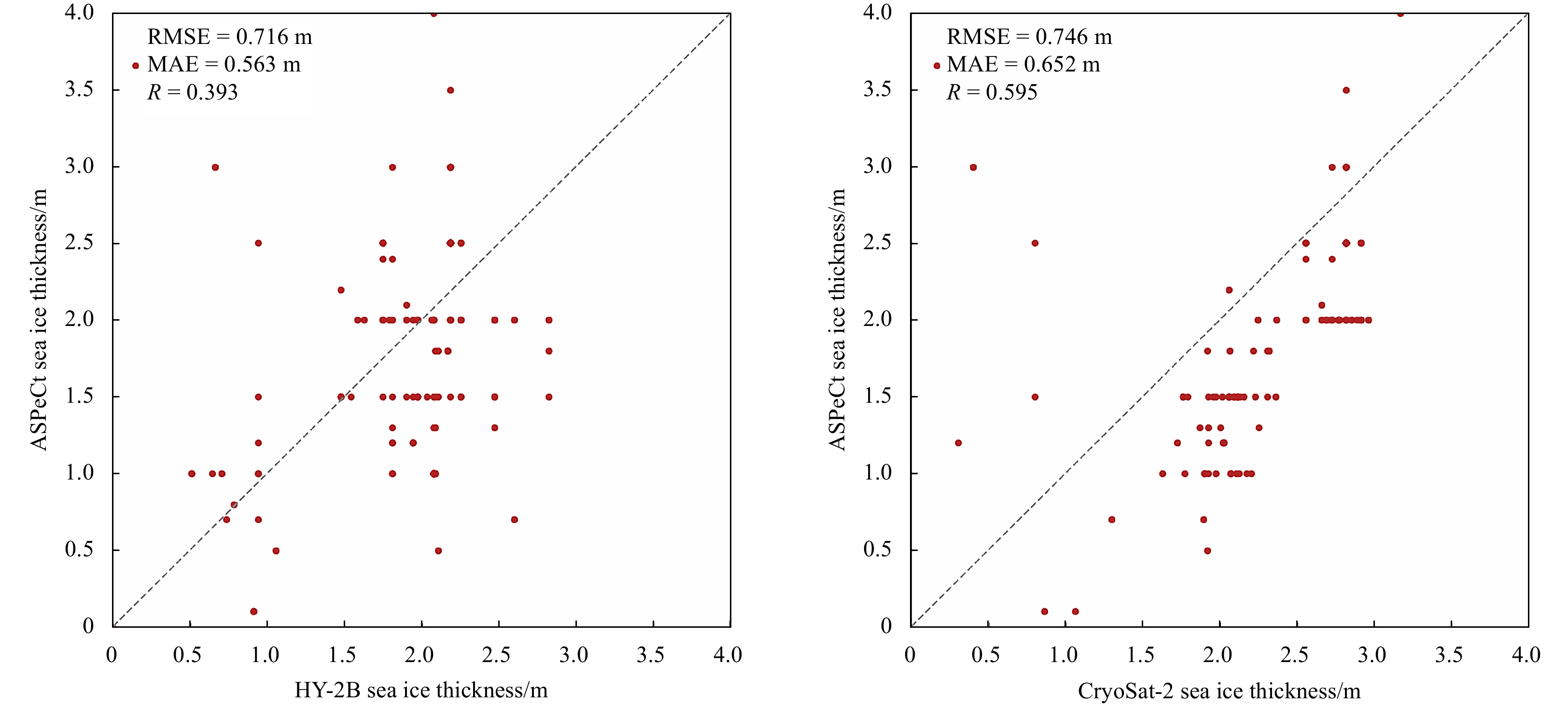
We also validated the HY-2B-derived sea ice thickness using in situ sea ice thickness measurements (Fig. 9). The root mean square error (RMSE) of the sea ice thickness estimated from the HY-2 satellite altimeter data in this study was 0.716 m, and the mean absolute error (MAE) value reached 0.563 m, which is slightly smaller than the CryoSat-2 result (0.746 m and 0.652 m, separately) while the CryoSat-2 result is better correlated. The HY-2B and CryoSat-2 derived sea ice thickness were slightly greater than the Antarctic Sea Ice Processes and Climate (ASPeCt) measured sea ice thickness; this may have been related to the underestimation tendency of ship-based sea ice thickness observations in a given area or grid because ships are always heading toward thin ice (Worby et al., 2008).
Figure
9.
Comparison of the sea ice thickness retrieved from HY-2 and CryoSat-2 altimeter data in this study and ship-based observations of sea ice thickness. RMSD, root-mean-square deviation; MAE, mean absolute error; R , correlation coefficient.
4.1
The influence of the HY-2B radar signal penetration interface on sea ice thickness retrieval
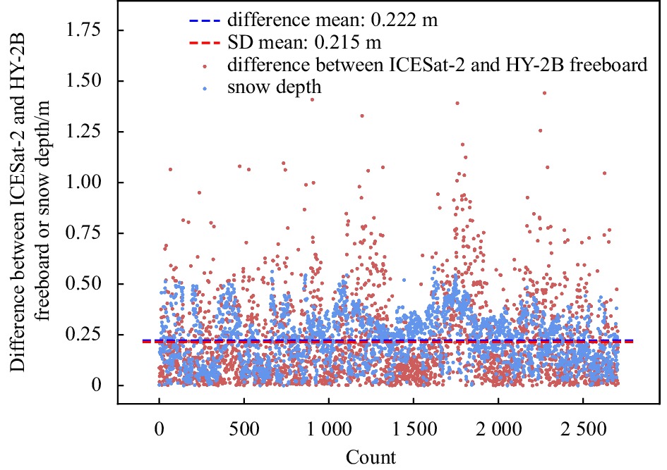
The penetration interface of radar altimetry signals is usually in the snow layer, indicating that radar altimetry signals do not always penetrate the snow fully on the surface of sea ice in Antarctica. In the sea ice freeboard calculation performed in this study, the radar altimetry signal was set as the default to complete snow penetration (Ricker et al., 2014). The penetration rate of the radar altimetry signal to snow is related to the humidity of the snow, the particle size and other factors, and the maximum penetration depth exceeds 20 cm according to a comparison with the laser altimetry freeboard (Ricker et al., 2014). In regard to specific altimeter satellites, the CryoSat-2 radar altimetry signal penetrates 96% of the snow layer on first-year sea ice and 82% on multiyear sea ice (Armitage and Ridout, 2015). The snow depth of AMSR2 demonstrated the presence of thick snow on sea ice in the Antarctic waters, especially in the coastal area where multiyear sea ice may exist. Theoretically, laser altimetry could sense the surface of the air-snow interface (Kwok et al., 2012), and the penetration depth could be explored by comparing the snow depth and the difference between the laser-derived freeboard and radar-derived freeboard in the case that the snow depth was known. Here, we used laser altimeter data (ICESat-2) and a snow depth product (AMSR2) to investigate the penetration of the HY-2B radar altimetry signals into snow. The difference between the ICESat-2 freeboard and HY-2B freeboard was calculated to explore the penetration of HY-2B through a snow depth comparison. Figure 10 shows that the mean value of difference between ICESat-2 and HY-2B freeboard was 0.215 m and the mean value of snow depth at the same location was 0.222 m. We believed that the snow depth obtained by AMSR2 is accurate, whereas the ICESat-2 reflection interface is at the snow surface, and the resulting difference in snow thickness of 0.007 m between these two results was mainly due to the penetrating ability of HY-2B to penetrate the snow. We chose as many grid cells as possible to reduce possible errors in individual data. The HY-2B radar altimetry signal penetrates 97% of the Antarctic snow layer, indicating that the penetration capability of the HY-2 satellite signal is slightly better than that of CryoSat-2. In addition, the radar signal penetration interface causes an overestimation of approximately 0.007 m in the Antarctic sea ice freeboard, resulting in an error of approximately 6 cm in the sea ice thickness calculations.
Figure
10.
Comparison of the differences between the ICESat-2 freeboard or HY-2B freeboard and AMSR2 snow depth.
4.2
Representativeness of valid sea ice thickness retrievals from HY-2B data
Li et al. (2018) reported that ICESat has 5%–20% valid sea ice thickness data compared to high-resolution sea ice concentration products, and there are several differences in the representativeness of ICESat data in different seas. HY-2B satellite data also suffer from a shortage of valid sea ice freeboard and thickness data. We counted the number of HY-2B sea ice thickness grid cells before interpolation and the number of grid cells with sea ice concentration higher than 0%, and then used their proportions to discuss the representativeness of the HY-2B data for the whole Antarctic waters and five sectors. Figure 11 shows the representativeness of the HY-2B sea ice freeboard and thickness retrievals for the whole Antarctic waters and five sectors. The mean rates of valid HY-2B grids at a 25-km resolution and the AMSR2 sea ice concentration were 22.25%, 15.8%, 26.27%, 25.15%, 28.21%, and 29.73% for the whole Antarctic waters, Weddell Sea, Indian Ocean, Pacific Ocean, Ross Sea, and Bellingshausen and Amundsen Seas, respectively. The Weddell Sea had the smallest effective ratio, while the Bellingshausen and Amundsen Seas had the largest ratios; this is exactly the opposite of the mean sea ice extent distribution. In addition, the minimum validity values for the six sea areas occurred from September to November, and the maximum values occurred in February, again in contrast to the sea ice extent trend. In summary, the sea ice thickness estimation performed in this study based on HY-2B satellite measurements could be considered most representative in the Bellingshausen and Amundsen Seas and least representative in the Weddell Sea, while the remaining sectors were similarly represented as the Bellingshausen and Amundsen Seas.
Figure
11.
Comparison of grid-cell counts in the Antarctic waters and five seas for the HY-2B sea ice thickness and sea ice concentration products.
4.3
Influence of different retracking algorithms on sea ice thickness retrievals
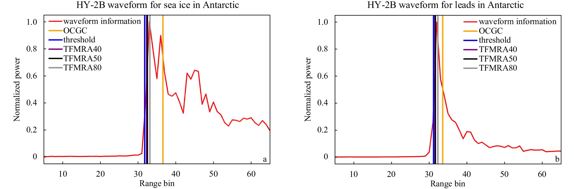
Waveform retracking algorithms play an important role in the determination of sea ice surface elevations (Helm et al., 2014). We chose the threshold first maximum retracker algorithm (TFMRA) and the threshold of 50% of the first-maximum power (TFMRA50) of the first maximum power, as in Helm et al. (2014), to achieve elevation correction and noise cancellation. We estimated that the surface elevation calculated by this method was closest to the snow-ice interface. The sea ice surface elevation plays a crucial part in the determination of the sea ice freeboard and thickness; thus, we compared the HY-2B-derived sea ice thickness based on commonly used retracking algorithms, including offset center of gravity retracker (OCOG), the threshold method and TFMRA methods (Helm et al., 2014). Figure 12 shows typical HY-2B waveforms for sea ice and leads and the locations of different retracking algorithms. The difference between the retracking methods is larger for sea ice than for leads, especially for OCGC, which is further proof that TFMRA is more suitable than conventional OCGC in the Antarctic waters.
Figure
12.
HY-2B original typical waveforms for sea ice (a) and leads (b) with colorful vertical lines that represent the different values of the retracking algorithm: orange (OCGC), blue (threshold algorithm), purple (TFMRA with 40% threshold), black (TFMRA with 50% threshold) and gray (TFMRA with 80% threshold).
We selected several tracks of HY-2B satellite data and accounted for the difference in sea ice freeboard through a comparison with the TFMRA50 retracking algorithm (Table 4). Compared to TFMRA50, TFMRA40, and the threshold method were more approximate, and the absolute deviation was less than 0.1 m. The derived sea ice freeboard and thickness of the OCGC and TFMRA80 algorithms differed more, and the absolute deviation was greater than 0.15 m, meaning that OCGC is the retracking algorithm that deviates the most from TFMRA50.
Table
4.
Effect of using different retracking algorithms on the sea ice freeboard estimations based on TFMRA50
4.4
Improvement and limitations for the retrieval of Antarctic sea ice thickness from HY-2B altimeter data
Satellite altimetry can provide sea ice elevation measurements in Antarctica when applied to retrieve the sea ice freeboard and thickness (Kurtz et al., 2014). Laser altimetry senses elevation at the air-snow interface, while radar altimetry senses elevation at the snow-ice interface, and sea ice freeboard and thickness can be estimated using the static equilibrium equation according to the sea ice-lead discrimination algorithm (Kwok and Kacimi, 2018). With regard to radar altimetry, the sea ice and lead discrimination algorithm is realized through the characteristic parameters of the radar altimetry signal (Kwok et al., 2019). At present, the lead discrimination and waveform retracking algorithms available for CryoSat-2 are relatively mature. Therefore, the CryoSat-2 radar altimetry algorithm can be used when applying HY-2B radar altimeter data for the retrieval of Antarctic sea ice freeboard and thickness.
This paper attempted to retrieve Antarctic sea ice thickness from HY-2B satellite altimeter data. A corresponding lead discrimination algorithm including new parameters confirmed by MODIS-derived leads was applied to estimate the Antarctic sea ice freeboard. Compared to existing algorithms used for radar altimetry satellites, the algorithm proposed in this study is more suitable for the HY-2B satellite. We applied the MODIS data corresponding to HY-2B to construct the lead classification rules. The classification rule-making error was one of the main sources of error in the derived sea ice freeboard and thickness results. The input parameters such as snow depth and density in the static equilibrium equation also affected the sea ice thickness calculation through Eq. (1) (Maksym and Markus, 2008; Xie et al., 2013). Notably, the HY-2B data had poor spatial coverage in the Antarctic waters, and there were many cavities between the HY-2B orbits, which is the reason why we chose to interpolate the sea ice freeboard grid to ensure spatial coverage. In addition, there were many invalid points with a lack of valid surface elevation or waveform data from the along-track perspective. We found more invalid measuring points in coastal areas than in offshore areas in the Antarctic waters, indicating that the former were likely to be better represented. There were more outliers in the HY-2B satellite data than in the other satellite data, including abnormally high or low surface elevation values of Antarctic sea ice. The HY-2B sea ice thickness retrieval algorithm relies on new and specialized lead classification rules based on corresponding MODIS-derived leads; however, it is expected to become a feasible alternative sea ice thickness-retrieval method in the Antarctic waters.
5.
Conclusions
The HY-2B satellite, carrying a radar altimeter, is available to provide surface elevation and waveform parameters for the retrieval of Antarctic sea ice freeboard and thickness. In this study, we designed an algorithm for the lead discrimination and retrieval of Antarctic sea ice freeboard and thickness from HY-2B satellite altimeter. We first applied MODIS IST products to extract leads and accessed them with matched Sentinel-1 SAR images; then, we generated a HY-2B decision tree for surface classification in the Antarctic waters based on the CART tree method. The Antarctic sea ice freeboard and thickness in 2019 were subsequently estimated, and we further analyzed their spatiotemporal characteristics. The retrieved Antarctic sea ice thickness was finally compared to the CryoSat-2 sea ice thickness and validated with the ASPeCt-measured sea ice thickness.
Compared to SAR images, the MODIS-extracted leads were capable of covering the whole Antarctic waters. Leads with large lengths and widths and relatively simple morphological features were easy to identify. The MODIS IST product caused some lead details to be missing when compared to Sentinel-1 SAR images. The lead classification accuracy for the HY-2B decision tree reached above 80%. The HY-2B-derived sea ice thickness in this study was thinner than the CryoSat-2 sea ice thickness, and the RMSE between the HY-2B-derived sea ice thickness and ASPeCt ship-based observed sea ice thickness was 0.62 m.
HY-2B penetrates snow relatively well and is representative at a scale of 25 km. It is worth noting that the choice of the retracking algorithm for the HY-2B waveform could also have a large impact on the sea ice freeboard and sea ice thickness estimations. Because the quality of extracted leads is compromised by the spatial resolution of MODIS images, obtaining high-quality and large-scale leads will be one of our main research directions for the accurate retrieval of Antarctic sea ice thickness in the future.
Acknowledgements:
We thank NSOAS for the HY-2B radar altimeter data, for the Sentinel-1 SAR image data, Alaska SAR Facility (ASF) NSIDC for the MODIS ice surface temperature data and ICESat-2 laser altimeter data, ESA for the CryoSat-2 data, and PANGAEA-Data Publisher for Earth & Environmental Science (PANGAEA) for the ship-based observed sea ice thickness data.
Armitage T W K, Davidson M W J. 2014. Using the interferometric capabilities of the ESA CryoSat-2 mission to improve the accuracy of sea ice freeboard retrievals. IEEE Transactions on Geoscience and Remote Sensing, 52(1): 529–536, doi: 10.1109/TGRS.2013.2242082
Armitage T W K, Ridout A L. 2015. Arctic sea ice freeboard from AltiKa and comparison with CryoSat-2 and operation IceBridge. Geophysical Research Letters, 42(16): 6724–6731, doi: 10.1002/2015GL064823
Chen Chuntao, Zhu Jianhua, Ma Chaofei, et al. 2021. Preliminary calibration results of the HY-2B altimeter’s SSH at China’s Wanshan calibration site. Acta Oceanologica Sinica, 40(5): 129–140, doi: 10.1007/s13131-021-1745-y
Comiso J C, Parkinson C L, Gersten R, et al. 2008. Accelerated decline in the Arctic sea ice cover. Geophysical Research Letters, 35(1): L01703
Crosta X, Kohfeld K E, Bostock H C, et al. 2022. Antarctic sea ice over the past 130 000 years—Part 1: a review of what proxy records tell us. Climate of the Past, 18(8): 1729–1756, doi: 10.5194/cp-18-1729-2022
Drüe C, Heinemann G. 2004. High-resolution maps of the sea-ice concentration from MODIS satellite data. Geophysical Research Letters, 31(20): L20403
Farrell S L, Markus T, Kwok R, et al. 2011. Laser altimetry sampling strategies over sea ice. Annals of Glaciology, 52(57): 69–76, doi: 10.3189/172756411795931660
Fons S W, Kurtz N T, Bagnardi M, et al. 2021. Assessing CryoSat-2 Antarctic snow freeboard retrievals using data from ICESat-2. Earth and Space Science, 8(7): e2021EA001728, doi: 10.1029/2021EA001728
Haas C, Lobach J, Hendricks S, et al. 2009. Helicopter-borne measurements of sea ice thickness, using a small and lightweight, digital EM system. Journal of Applied Geophysics, 67(3): 234–241, doi: 10.1016/j.jappgeo.2008.05.005
Helm V, Humbert A, Miller H. 2014. Elevation and elevation change of Greenland and Antarctica derived from CryoSat-2. The Cryosphere, 8(4): 1539–1559, doi: 10.5194/tc-8-1539-2014
Holland M M, Bitz C M, Hunke E C, et al. 2006. Influence of the sea ice thickness distribution on polar climate in CCSM3. Journal of Climate, 19(11): 2398–2414, doi: 10.1175/JCLI3751.1
Jia Yongjun, Yang Jungang, Lin Mingsen, et al. 2020. Global assessments of the HY-2B measurements and cross-calibrations with Jason-3. Remote Sensing, 12(15): 2470, doi: 10.3390/rs12152470
Jiang Chengfei, Lin Mingsen, Wei Hao. 2019. A study of the technology used to distinguish sea ice and seawater on the Haiyang-2A/B (HY-2A/B) altimeter data. Remote Sensing, 11(12): 1490, doi: 10.3390/rs11121490
Kern S, Khvorostovsky K, Skourup H, et al. 2015. The impact of snow depth, snow density and ice density on sea ice thickness retrieval from satellite radar altimetry: results from the ESA-CCI Sea Ice ECV Project Round Robin Exercise. The Cryosphere, 9(1): 37–52, doi: 10.5194/tc-9-37-2015
Kurtz N T, Galin N, Studinger M. 2014. An improved CryoSat-2 sea ice freeboard retrieval algorithm through the use of waveform fitting. The Cryosphere, 8(4): 1217–1237, doi: 10.5194/tc-8-1217-2014
Kurtz N T, Markus T. 2012. Satellite observations of Antarctic sea ice thickness and volume. Journal of Geophysical Research: Oceans, 117(C8): C08025
Kurtz N T, Markus T, Cavalieri D J, et al. 2009. Estimation of sea ice thickness distributions through the combination of snow depth and satellite laser altimetry data. Journal of Geophysical Research: Oceans, 114(C10): C10007
Kwok R. 2010. Satellite remote sensing of sea-ice thickness and kinematics: a review. Journal of Glaciology, 56(200): 1129–1140, doi: 10.3189/002214311796406167
Kwok R, Cunningham G F, Manizade S S, et al. 2012. Arctic sea ice freeboard from IceBridge acquisitions in 2009: Estimates and comparisons with ICESat. Journal of Geophysical Research: Oceans, 117(C2): C02018
Kwok R, Kacimi S. 2018. Three years of sea ice freeboard, snow depth, and ice thickness of the Weddell Sea from Operation IceBridge and CryoSat-2. The Cryosphere, 12(8): 2789–2801, doi: 10.5194/tc-12-2789-2018
Kwok R, Kacimi S, Markus T, et al. 2019. ICESat-2 surface height and sea ice freeboard assessed with ATM Lidar acquisitions from operation IceBridge. Geophysical Research Letters, 46(20): 11228–11236, doi: 10.1029/2019GL084976
Kwok R, Kacimi S, Webster M A, et al. 2020. Arctic snow depth and sea ice thickness from ICESat-2 and CryoSat-2 freeboards: A first examination. Journal of Geophysical Research: Oceans, 125(3): e2019JC016008, doi: 10.1029/2019JC016008
Landy J C, Petty A A, Tsamados M, et al. 2020. Sea ice roughness overlooked as a key source of uncertainty in CryoSat-2 ice freeboard retrievals. Journal of Geophysical Research: Oceans, 125(5): e2019JC015820, doi: 10.1029/2019JC015820
Landy J C, Tsamados M, Scharien R K. 2019. A facet-based numerical model for simulating SAR altimeter echoes from heterogeneous sea ice surfaces. IEEE Transactions on Geoscience and Remote Sensing, 57(7): 4164–4180, doi: 10.1109/TGRS.2018.2889763
Laxon S W, Giles K A, Ridout A L, et al. 2013. CryoSat-2 estimates of Arctic sea ice thickness and volume. Geophysical Research Letters, 40(4): 732–737, doi: 10.1002/grl.50193
Laxon S, Peacock N, Smith D. 2003. High interannual variability of sea ice thickness in the Arctic region. Nature, 425(6961): 947–950, doi: 10.1038/nature02050
Lee S, Im J, Kim J, et al. 2016. Arctic sea ice thickness estimation from CryoSat-2 satellite data using machine learning-based lead detection. Remote Sensing, 8(9): 698, doi: 10.3390/rs8090698
Lee Y K, Kongoli C, Key J. 2015. An in-depth evaluation of heritage algorithms for snow cover and snow depth using AMSR-E and AMSR2 measurements. Journal of Atmospheric and Oceanic Technology, 32(12): 2319–2336, doi: 10.1175/JTECH-D-15-0100.1
Lewis R J. 2000. An introduction to classification and regression tree (CART) analysis. In: Presented at the 2000 Annual Meeting of the Society for Academic Emergency Medicine in San Francisco, California (Vol. 14). Torrance: Department of Emergency Medicine Harbor-UCLA Medical Center
Li Wanwu, Liu Lin, Zhang Jixian. 2021. Fusion of SAR and optical image for sea ice extraction. Journal of Ocean University of China, 20(6): 1440–1450, doi: 10.1007/s11802-021-4824-y
Li Huan, Xie Hongjie, Kern S, et al. 2018. Spatio-temporal variability of Antarctic sea-ice thickness and volume obtained from ICESat data using an innovative algorithm. Remote Sensing of Environment, 219: 44–61, doi: 10.1016/j.rse.2018.09.031
Maksym T, Markus T. 2008. Antarctic sea ice thickness and snow-to-ice conversion from atmospheric reanalysis and passive microwave snow depth. Journal of Geophysical Research: Oceans, 113(C2): C02S12
Markus T, Cavalieri, D J. 1998. Snow depth distribution over sea ice in the Southern Ocean from satellite passive microwave data. Antarctic sea ice: physical processes, interactions and variability, 74, 19-39
Markus T, Neumann T, Martino A, et al. 2017. The Ice, Cloud, and land Elevation Satellite-2 (ICESat-2): Science requirements, concept, and implementation. Remote Sensing of Environment, 190: 260–273, doi: 10.1016/j.rse.2016.12.029
Ozsoy-Cicek B, Ackley S, Xie Hongjie, et al. 2013. Sea ice thickness retrieval algorithms based on in situ surface elevation and thickness values for application to altimetry. Journal of Geophysical Research: Oceans, 118(8): 3807–3822, doi: 10.1002/jgrc.20252
Passaro M, Müller F L, Dettmering D. 2018. Lead detection using Cryosat-2 delay-doppler processing and Sentinel-1 SAR images. Advances in Space Research, 62(6): 1610–1625, doi: 10.1016/j.asr.2017.07.011
Reiser F, Willmes S, Heinemann G. 2020. A new algorithm for daily sea ice lead identification in the Arctic and Antarctic winter from thermal-infrared satellite imagery. Remote Sensing, 12(12): 1957, doi: 10.3390/rs12121957
Ricker R, Hendricks S, Helm V, et al. 2014. Sensitivity of CryoSat-2 Arctic sea-ice freeboard and thickness on radar-waveform interpretation. The Cryosphere, 8(4): 1607–1622, doi: 10.5194/tc-8-1607-2014
Shi Lijian, Karvonen J, Cheng Bin, et al. 2014. Sea ice thickness retrieval from SAR imagery over Bohai Sea. In: 2014 IEEE Geoscience and Remote Sensing Symposium. Quebec City: IEEE, 4864–4867
Spreen G, Kern S, Stammer D, et al. 2006. Satellite-based estimates of sea-ice volume flux through Fram Strait. Annals of Glaciology, 44: 321–328, doi: 10.3189/172756406781811385
Tian Liuxi, Xie Hongjie, Ackley S F, et al. 2020. Sea-ice freeboard and thickness in the Ross Sea from airborne (IceBridge 2013) and satellite (ICESat 2003–2008) observations. Annals of Glaciology, 61(82): 24–39, doi: 10.1017/aog.2019.49
Turner J, Comiso J C, Marshall G J, et al. 2009. Non-annular atmospheric circulation change induced by stratospheric ozone depletion and its role in the recent increase of Antarctic sea ice extent. Geophysical Research Letters, 36(8): L08502
Wang Jinfei, Min Chao, Ricker R, et al. 2022. A comparison between Envisat and ICESat sea ice thickness in the Southern Ocean. The Cryosphere, 16(10): 4473–4490, doi: 10.5194/tc-16-4473-2022
Wang Xianwei, Xie Hongjie, Ke Yanan, et al. 2013. A method to automatically determine sea level for referencing snow freeboards and computing sea ice thicknesses from NASA IceBridge airborne LIDAR. Remote Sensing of Environment, 131: 160–172, doi: 10.1016/j.rse.2012.12.022
Weissling B P, Lewis M J, Ackley S F. 2011. Sea-ice thickness and mass at Ice Station Belgica, Bellingshausen Sea, Antarctica. Deep-Sea Research Part II: Topical Studies in Oceanography, 58(9/10): 1112–1124, doi: 10.1016/j.dsr2.2010.10.032
Williams G, Maksym T, Wilkinson J, et al. 2015. Thick and deformed Antarctic sea ice mapped with autonomous underwater vehicles. Nature Geoscience, 8(1): 61–67, doi: 10.1038/ngeo2299
Willmes S, Heinemann G. 2015. Pan-Arctic lead detection from MODIS thermal infrared imagery. Annals of Glaciology, 56(69): 29–37, doi: 10.3189/2015AoG69A615
Worby A P, Geiger C A, Paget M J, et al. 2008. Thickness distribution of Antarctic sea ice. Journal of Geophysical Research: Oceans, 113(C5): C05S92
Worby A P, Steer A, Lieser J L, et al. 2011. Regional-scale sea-ice and snow thickness distributions from in situ and satellite measurements over East Antarctica during SIPEX 2007. Deep-Sea Research Part II: Topical Studies in Oceanography, 58(9/10): 1125–1136, doi: 10.1016/j.dsr2.2010.12.001
Xie Hongjie, Ackley S F, Yi Donghui, et al. 2011. Sea-ice thickness distribution of the Bellingshausen Sea from surface measurements and ICESat altimetry. Deep-Sea Research Part II: Topical Studies in Oceanography, 58(9/10): 1039–1051, doi: 10.1016/j.dsr2.2010.10.038
Xie Hongjie, Tekeli A E, Ackley S F, et al. 2013. Sea ice thickness estimations from ICESat altimetry over the Bellingshausen and Amundsen Seas, 2003–2009. Journal of Geophysical Research: Oceans, 118(5): 2438–2453, doi: 10.1002/jgrc.20179
Yi Donghui, Zwally H J, Robbins J W. 2011. ICESat observations of seasonal and interannual variations of sea-ice freeboard and estimated thickness in the Weddell Sea, Antarctica (2003–2009). Annals of Glaciology, 52(57): 43–51, doi: 10.3189/17275641 1795931480
Zhang Xi, Zhu Yixun, Zhang Jie, et al. 2021. Assessment of Arctic sea ice classification ability of Chinese HY-2B dual-band radar altimeter during winter to early spring conditions. IEEE Journal of Selected Topics in Applied Earth Observations and Remote Sensing, 14: 9855–9872, doi: 10.1109/JSTARS.2021.3114228
Zhong Wenqing, Jiang Maofei, Xu Ke, et al. 2023. Arctic sea ice lead detection from Chinese HY-2B radar altimeter data. Remote Sensing, 15(2): 516, doi: 10.3390/rs15020516
Zwally H J, Yi Donghui, Kwok R, et al. 2008. ICESat measurements of sea ice freeboard and estimates of sea ice thickness in the Weddell Sea. Journal of Geophysical Research: Oceans, 113(C2): C02S15
Figure 1. Five sea areas of the Antarctic waters, with an overlaid background of the maximum (blue, September 20, 2019) Antarctic sea ice extent in 2019. The whole Antarctic waters refers to the sea areas around the Antarctic continent within latitudes above 60°S.
Figure 2. MODIS-derived ice surface temperature on September 29, 2019, with a cloud mask (yellow) and Antarctic continent (gray). Arrow 1 refers to the area with a lead, and Arrow 2 represents an area of invalid values (cloud).
Figure 3. Geometric relationships among the sea ice freeboard ($ {h}_{\mathrm{i}} $), snow depth (${h}_{\mathrm{s}}$) and sea ice thickness ($ {h}_{\mathrm{i}} $) measured by the HY-2B radar satellite altimeter.
Figure 4. Comparison between the ice surface temperature and extracted leads on October 3, 2019: a. MODIS-derived ice surface temperature with cloud mask (yellow) and b. MODIS-derived leads with cloud mask (yellow).
Figure 5. Example of Sentinel-1 SAR images and corresponding MODIS-extracted leads on October 6, 2019: a. Sentinel-1 SAR images and b. MODIS-extracted leads.
Figure 6. HY-2B surface classification decision tree in Antarctica.
Figure 7. Antarctic sea ice thickness retrieved from HY-2B satellite altimeter data in 2019 (a) and average sea ice thickness by month in 2019 (b).
Figure 8. Comparison between the HY-2B sea ice thickness and CryoSat-2 sea ice thickness in the whole Antarctic waters (a), Weddell Sea (b), Indian Ocean (c), Pacific Ocean (d), Ross Sea (e) and Bellingshausen and Amundsen Seas (f). RMSD, root-mean-square deviation; MAE, mean absolute error; R, correlation coefficient.
Figure 9. Comparison of the sea ice thickness retrieved from HY-2 and CryoSat-2 altimeter data in this study and ship-based observations of sea ice thickness. RMSD, root-mean-square deviation; MAE, mean absolute error; R , correlation coefficient.
Figure 10. Comparison of the differences between the ICESat-2 freeboard or HY-2B freeboard and AMSR2 snow depth.
Figure 11. Comparison of grid-cell counts in the Antarctic waters and five seas for the HY-2B sea ice thickness and sea ice concentration products.
Figure 12. HY-2B original typical waveforms for sea ice (a) and leads (b) with colorful vertical lines that represent the different values of the retracking algorithm: orange (OCGC), blue (threshold algorithm), purple (TFMRA with 40% threshold), black (TFMRA with 50% threshold) and gray (TFMRA with 80% threshold).


 DownLoad:
 DownLoad: