Combined effect of subsurface dam and layered heterogeneity on groundwater flow and salinity distribution in stratified coastal aquifers

1. Introduction

According to a report by Vörösmarty et al. (2010), around 80% of the global population is confronted with significant issues of water scarcity and water pollution. Sea level increases and groundwater overexploitation in coastal areas, which often leads to a decrease in the hydraulic gradient in coastal areas (Shen et al., 2020; Werner et al., 2013). This caused seawater to flow into coastal freshwater aquifers under ocean forcing (e.g., tides, waves), which is commonly called saltwater intrusion. Saltwater intrusion is a phenomenon that widely occurs in many parts of the world. In addition to polluting freshwater resources and significantly decreasing their availability (Tang et al., 2021a, b), saltwater intrusion can also result in soil salinization and hinder industrial and agricultural productivity in coastal wetlands (Fang et al., 2021b; Chang et al., 2019). Thus, it is crucial to have a better comprehension of saltwater intrusion and successfully reduce freshwater contamination is essential for managing water resources, economic development, and human health in coastal areas.

To protect freshwater resources, some researchers have developed various strategies, such as diminishing the extraction of freshwater and preventing the influx of saltwater (by extracting saltwater and constructing subsurface barriers) (Christy and Lakshmanan, 2017; Botero-Acosta and Donado, 2015). It has been reported that subsurface barriers are a technically feasible way to prevent saltwater intrusion as well as increase of freshwater storage. Subsurface barriers are constructed by injecting impervious materials into underground aquifers (Abdoulhalik and Ahmed, 2017). Many coastal countries have built a series of subsurface physical barriers to solve the saltwater intrusion problem since the 1980s (Zheng et al., 2020; Abdoulhalik et al., 2017; Lalehzari and Tabatabaei, 2015). For example, subsurface physical barriers for preventing saltwater intrusion were used in Sardinia as early as the Roman Empire era (Hanson and Nilsson, 1986). Approximately 15 submarine barriers were constructed in Japan to store and regulate freshwater for reliable extraction, and approximately seven subsurface barriers were implemented to mitigate saltwater intrusion (Luyun et al., 2009). To control saltwater intrusion, China has constructed subsurface physical barriers in the coastal cities of Shandong Province (such as Longkou, Qingdao, Yantai, and Rizhao) (Kang et al., 2021; Fang et al., 2020; Zeng et al., 2018; Kang and Xu, 2017). Currently, there exist three primary types (Fang et al., 2021b; Kaleris and Ziogas, 2013): (1) subsurface dam, where a gap is maintained in the upper section of the aquifer to allow freshwater release; (2) cutoff wall, which features an opening at the base of the aquifer for freshwater discharge; and (3) fully penetrating barriers, spanning from the top to the bottom of aquifers. Subsurface dams, out of the three categories, prove to be the most extensively employed and effective technique in addressing the issue of saltwater intrusion (Chang et al., 2022; Zheng et al., 2022).

Studies conducted in the last ten years, both experimental and numerical, have demonstrated the impact of subsurface dams on groundwater flow and salinity distribution in coastal aquifers (Fang et al., 2023, 2021b). According to a study conducted in Chang et al. (2019), it was discovered that subsurface dams can effectively control saltwater intrusion even when their height is slightly lower than the height of the saltwater wedge (SW). As a result, they suggested and implemented subsurface dams with the minimum effective height to control saltwater intrusion. Zheng et al. (2021) note that fully removing residual saltwater remaining in the field after subsurface dam construction can take several decades. While previous research has shown the efficacy of underground dams, they mainly utilized static sea boundary conditions and overlooked tidal-induced fluctuations in the oceanic water table. In fact, tidal fluctuations can lead to dynamic and complicated groundwater flow and salinity distribution patterns in coastal aquifers (Kong et al., 2023; Fang et al., 2023). SWs and upper saline plumes (USPs) can develop when tides are present, caused by the recirculation of saltwater driven by density and induced by the tide (Gao et al., 2023; Kong et al., 2023; Fang et al., 2021a). Freshwater driven by inland hydraulic gradients bypasses USP and SW flows into nearshore aquifers and mixes with saltwater infiltrating across sea beaches (Fang et al., 2023). Therefore, Fang et al. (2021b) examined the impacts of varying dam heights, locations, and dispersivity. The findings indicated that the minimum viable height was approximately 95% of the SW height (the height of the SW determined by the 95% isolines before the construction of the dam) in the absence of tidal conditions and 20% of the SW height when tides were present. Song et al. (2022) investigated the effects of physical barriers on coastal aquifer recovery after storm surges and found that physical barriers expanded salinization volume and total salt volume and prolonged aquifer recovery. Fang et al. (2023) demonstrated that subsurface dams change the location of the freshwater discharge at the aquifer-sea interface, fresh and saline submarine groundwater discharge fluxes peaked at the minimum effective height.

A substantial common limitation of the aforementioned studies is that they considered homogeneous and isotropic coastal aquifers. However, inherent subsurface heterogeneity is inevitable within geological formations, and numerous coastal aquifers exhibit stratification and commonly contain low-permeability layers (LPLs) that are confined between layers of high permeability (Gao et al., 2022; Ratner-Narovlansky et al., 2020; Li and Boufadel, 2010), which may impact the dynamic processes of groundwater flow and salinity distribution to various degrees (Werner et al., 2013). For example, the stratified coastal aquifer at Southern Oahu, Hawaii by Oki et al. (1998) reported that a lower-permeability mud layer exists between the upper and the lower high-permeability, and they found that the thickness of the LPL was approximately 30% of the three-layered aquifer configuration. Ratner-Narovlansky et al. (2020) reported that a lower permeable clay layer distribution between the upper and the lower high-permeability sand layers at the Dor Bay (Israel) coastal aquifer. Many experimental and numerical studies have demonstrated the impact of LPL on the groundwater flow and the dispersion of salt in coastal aquifers. Abdoulhalik and Ahmed (2017) investigated the relationship between the four different configurations and subsurface dam resistance efficiency against saltwater intrusion in a laboratory-scale aquifer. The discovery was made that the existence of an LPL in the higher section of shoreline may enhance the ability of subsurface dams to prevent saltwater intrusion under static sea boundary conditions. The impact of an LPL on finger flow patterns and land-sourced solute transport in coastal aquifers was investigated in a study conducted by Zhang et al. (2021). Their results indicated that LPL has the ability to greatly decrease the dimensions and expedite the development of salt fingers linked to unstable USP. Gao et al. (2022) showed that the stratification pattern disrupts groundwater flow, and the existence of a low permeability layer within the aquifer increases the area of nitrate-contaminated zones and nitrate quality.

To our knowledge, the combined impact of subsurface dams and tides on the flow of groundwater and the distribution of salinity in unconfined aquifers with stratification is still uncertain, despite previous research revealing the separate effects of these factors. In order to fill this research gap, we conducted numerical simulations based on a conceptual 2-dimension cross-shore section of a three-layered coastal aquifer with an LPL. In particular, this study aimed to address the following key questions: (1) How do subsurface dams and aquifer stratification jointly affect the salinity distribution in coastal unconfined aquifers; (2) How groundwater flow and circulation are altered; and (3) How important are the penetration depth and location of subsurface dams. The research outcomes would promote a more comprehensive understanding of the complex hydrodynamics in layered coastal aquifers, and provide decisive guidance for the design of subsurface dams aimed at both saltwater intrusion control.

2. Numerical model

2.1 Governing equations and boundary conditions

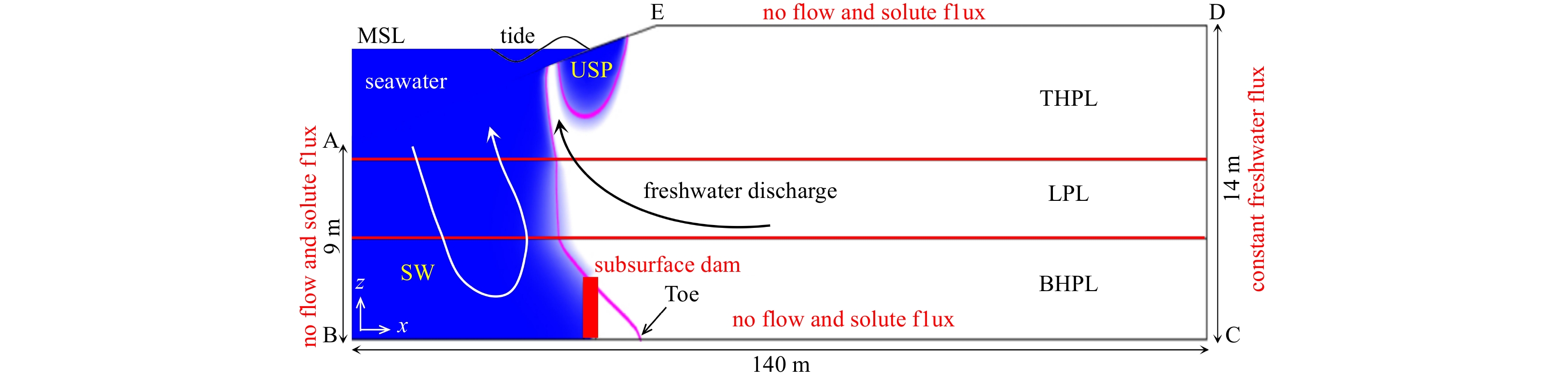
Based on the research conducted by Ratner-Narovlansky et al. (2020) at the Dor Bay (Israel) coastal aquifer, the LPL extends over 150 m towards the sea. The ABCDE model domain depicts a 2-dimension cross-shore section of this aquifer (Fig. 1d), where AE represents the marsh platform. A 2-dimension variably saturated model was developed by using COMSOL Multiphysics to simulate groundwater flow and solute transport in a beach aquifer by solving the 2-dimension Richard’s equation.

Figure  1.  Conceptual and numerical model schematic showing a layered coastal aquifer with a low-permeability layer (LPL), a top high-permeability layer (THPL), and a bottom high-permeability layer (BHPL). The upper saline plume (USP), the saltwater wedge (SW), the freshwater discharge zone, the saltwater wedge toe (Toe), and the mean sea level (MSL) are shown. The Toe represents the point where the x-axis intersects with the contour line of 50% salinity, and magenta lines indicate the 50% salinity contour before the construction of a subsurface dam. And red lines represent the subsurface dams, the black lines with arrows indicate the freshwater circulation patterns, and the white lines with arrows indicate the density-driven recirculation patterns. The coordinates of boundary nodes are A (0 m, 9 m), B (0 m, 0 m), C (140 m, 0 m), D (140 m, 14 m), and E (50 m, 14 m).

DownLoad: Full-Size Img PowerPoint

where ρ is fluid density (kg/m³); p is the pressure (Pa); z is the elevation head (m); k_s is the saturated permeability (m/s); k_r is the relative permeability (m/s); c_m is the specific moisture capacity (m⁻¹); S_e is the effective saturation; S is the storage coefficient; g is the acceleration of gravity (9.81 m/s²); and μ is dynamic viscosity (Pa·s); $\nabla $ is the gradient operator.

The constitutive relationships between k_s, k_r and soil hydraulic properties were described by the equations of van Genuchten (1980):

where m = 1 − (1/n), α and n obey van Genuchten (1980) model, describes the shape of both the moisture (m⁻¹) and relative permeability functions; K is hydraulic conductivity (m/s); θ is the water content; θ_s and θ_r are the saturated and the residual water contents of the porous medium, respectively.

The boundary conditions for pore water flow are as following:

For ocean boundary AE, a semipervious layer or seepage face boundary condition (Eqs (6) and (7)) was assigned to the marsh platform boundary representing the sediment-water or sediment-atmosphere interface, including the intertidal zone (please refer to Jiang et al. (2021) and Shen et al. (2019) for details):

where n is the unit vector normal to the interface (pointing outward); q is the Darcy velocity (m/s); the total head is H and above sea level is H_b (m); R_b is the conductive term (s⁻¹); K_h is the saturated hydraulic conductivity (m/s) and a coupling length scale (L). To handle the boundary conditions effectively, two conditions have been taken into account. The head difference is determined by the disparity between the overlying seawater and the beach interface when the aquifer is fully saturated and the external head (H_b) is above the elevation head at sea level. If the overall elevation (H) surpasses the level of the ocean (H_b) and the pressure elevation is equivalent to or greater than the atmospheric pressure, the boundary will be classified as a seepage surface. When the aquifer is not saturated, if the value of R_b is equal to zero, the boundary becomes a no-flow boundary. The node salinity is determined by the velocity of the groundwater. When the velocity is directed towards the center, the estimation of salinity is based on the salinity of seawater. Alternatively, the salinity of the groundwater in the vicinity of the node is utilized. Previous research has shown that this modeling technique is valuable for explaining the fluctuation of water levels and the duration of stay in the transition zone (Shen et al., 2019; Xin et al., 2010).

Applying a time-varying Dirichlet boundary condition (Eq. (8)), a tidal signal is imposed on the interface nodes:

where the tidal head (h(t)) is determined by the time t (h); the mean sea level (MSL) is 13 m; the tidal amplitudes (A) is 0.5 m; and the tidal cycle (T) is a semidiurnal tide (12 h). The water flow boundary conditions are depicted as follow (Fig. 1).

Boundary CD is the inland boundary was assigned a constant freshwater flux:

where Q_fresh represents a consistent influx of fresh groundwater (0.5 m²/d).

Boundary AB, BC, DE are the no-flow boundary conditions:

The equation describes the transport of solute in porous media with species:

where C is salinity (35), which was adopted from Robinson et al. (2018) and Shen et al. (2019); D_H is the hydrodynamic dispersion coefficient (m²/s), ${{\partial \rho } / {\partial {C_{{\text{salt}}}}}}$ is a constant (0.714 3), ρ₀ = 1 000 kg/m³.

The boundary conditions (Fig. 1) for solute transport are as following.

Ocean boundary AE:

Boundary CD is the inland boundary conditions:

Boundary AB, BC, DE:

where $ {C}_{\text{salt},0}\left(x,z,t\right) $ is kept constant over time in investigating the effect of invariable salt input concentration on the cycling in the coastal as suggested by previous studies (Jiang et al., 2022; Heiss, 2020; Anwar et al., 2014). These parameters and boundaries are consistent with those reported previous studies (Anwar et al., 2014; Spiteri et al., 2008b).

2.2 Model parameters and simulations

This study considered one homogeneous case and one layered case with an LPL. The model area has a depth of 14 m and a beach boundary that slopes at a rate of 0.1 (refer to Fig. 1). This was similar to a standard aquifer system found in sandy coastal areas (Carsel and Parrish, 1988). In the case where K is 15 m/d, the porosity is 0.25, and the longitudinal dispersion coefficient (α_L) and transverse dispersion coefficient (α_T) are 0.2 m and 0.02 m, respectively (Anwar et al., 2014). The van Genuchten (1980) equations utilized a residual saturation (S_e) value of 0.1, with the parameters α and n assigned as 14.5 m⁻¹ and 2.68, correspondingly. Previous research on aquifer groundwater flow and solute transport (Shen et al., 2019) has utilized the residual saturation, α, and n. In the case-layered scenario, the K value of the LPL was established at 1.5 m/d, which was ten times lower than the upper and lower layers in the same scenario. To keep things simple, the values of additional hydrological parameters such as residual saturation (S_e), α, and n, as well as longitudinal (α_L) and transverse (α_T), remained constant for both low and high permeability layer. Furthermore, the salinity and density were adjusted to 35 and 1 025 kg/m³, correspondingly. The freshwater salinity is 0 and the density is 1 000 kg/m³ (refer to Table 1).

Table  1.  Particle travel times and starting position

Starting position	Particle travel time
	Tide-no LPL-no dam	Tide-LPL-no dam	Tide-no LPL-dam	Tide-LPL-dam
x = 5 m, z = 9.5 m	2 973.4 d	2 638.9 d	2 906.1 d	2 537.0 d
x = 15 m, z = 10.5 m	1 071.0 d	2 152.7 d	1 288.9 d	1 998.8 d
x = 25 m, z = 11.5 m	411.1 d	1 071.6 d	377.3 d	1 043.6 d
x = 140 m, z = 2 m	537.9 d	627.2 d	535.0 d	621.5 d
x = 140 m, z = 6 m	511.8 d	1 284.9 d	513.0 d	1 278.2 d
x = 140 m, z = 10 m	495.3 d	483.1 d	494.2 d	485 d
Note: x and z are the horizontal and vertical coordinate values, respectively.

 | Show Table

DownLoad: CSV

The subsurface dam had a thickness of 2 m, and the sections occupied by the dam were designated as having low permeability (one thousand times less than the permeability of the sand, 1.5 × 10⁻⁴ m/d). The LPL had a thickness of 3.5 m, which accounted for approximately 30% of the MSL. After the validation of the numerical model by Fang et al. (2021a) experimental cases, a range of experimental scenarios were tested to assess their impact on controlling saltwater intrusion and freshwater discharge. These scenarios included no-layered-no-dam, no-layered-dam, layered-no-dam, and layered-dam cases. Later on, based on case-layered, a sensitivity analysis was conducted to explore the effects of subsurface dam heights and locations, the LPL on saltwater intrusion control and freshwater discharge in the LPL-bearing coastal aquifer.

Simulations were conducted using a time interval of 100 s, and the density of the mesh was enhanced along the shoreline, ensuring a minimum Δx measurement of 6 cm. To avoid numerical oscillation, we ensured the Courant did not exceed 1, and Péclet number (P_e) criterion to ensure the numerical stability (Voss and Souza, 1987):

where ΔL (m) represents the distance of freshwater flow between two sides of an element.

2.3 Measurable diagnostics

Parameter λ represents the evaluation of a subsurface dam’s effectiveness through the rate of change in the location of the toe:

where Toe₀ and Toe_i were the steady-state saltwater toe locations before and after the construction of a subsurface dam (m). It was measured by the position of 50% salinity interfaces.

To further quantify the impact of subsurface dams on the discharge of freshwater, the variation of the total freshwater flux (emission flux), across the beach is calculated as follows:

where B (m) is the unit width of the beach, q_out (m²/d) is the outward Darcy flux. The length of the upwelling area (l_out) for the outflow are evaluated as description in previous studies (Jiang et al., 2022, 2020; Singh et al., 2019).

In order to calculate the time (t_r) for the natural removal of residual saltwater after installation of the subsurface dams, we used the 0.1×Toe reduced time to assess, thus defined 0.1×Toe as the value of the intersection point between the 10% salinity isoline of the saline wedge and the x-axis.

3. Results

3.1 Model calibration

The flume experiments of Fang et al. (2021a) were conducted over a homogeneous aquifer with a fixed water depth of 0.245 m, the tank dimensions were 1.729 m (length) × 0.45 m (height) × 0.08 m (width). Similar to the experiments of Fang et al. (2021a), we conducted a numerical simulation as follows: for one set, examined the impact of tide regimes on saltwater intrusion. A subsurface dam was included in the second set, which was designed to work with the tidal patterns. The subsurface dam was located at x = 0.395 m, then the subsurface dam location was set to x = 0.6 m. The average elevation of the ocean surface is 0.238 m above the sand tank’s foundation. The predetermined tidal range is 0.02 m, the tidal period preset to 1 min, the α_L was 0.001 m, and the transverse dispersivity (α_T) was set at 1/10 of α_L. These parameters are consistent with Fang et al. (2021a), readers may refer to Fang et al. (2021a) for more details on the parameter values and experiment methods.

Figure 2 shows the numerical simulation results for the experimental of Fang et al. (2021a) cases. The predicted salinities matched well with the measurement for all cases. The solid white lines represented the 50% isohalines. Traditionally, 50% isohalines were used to determine the salt-freshwater interface (Kuan et al., 2012). Hydraulic gradients caused by tidal oscillations result in the infiltration of saltwater near the high tide mark and discharge near the low tide mark, which is separated from the SW by a freshwater discharge zone, forming a USP, these findings align with previous research conducted by Gao et al. (2023), Kong et al. (2023), Santos et al. (2021), and Heiss (2020). As shown in the experiments, the saltwater intrusion distance was 0.73 m in the case Tide-no-dam (Toe = 0.73 m). However, by implementing a subsurface dam with a location set at x = 0.395 m and a height of 0.13 m, the intrusion of saltwater was effectively prevented, and the saltwater intrusion distance was controlled at the dam location with an SW height of 0.08 m, i.e., the saltwater intrusion distance decreased from 0.730 m to 0.395 m after the construction of a subsurface dam. Moving the subsurface dam further inland, the saltwater intrusion distance again was controlled at the dam location, the Toe increased from 0.395 m to 0.600 m (Figs 2a2 and 2a3). The SW height (0.065 m) was much smaller than the dam height, compared to that in Fig. 2a2.

Figure  2.  Experimental (a) (Fang et al., 2021a) and our modelled (b) salinity distributions in the intertidal beach aquifer under conditions of tide and no-dam, tide and dam. The horizontal dash lines are high tide and low tide levels, solid white lines indicated numerical results for 50% salinity contours isohalines by Fang et al. (2021a), and solid black lines indicated 50% salinity contours isohalines in this numerical results. USP: upper saline plume; SW: the saltwater wedge. x and z are the horizontal and vertical coordinate values, respectively.

DownLoad: Full-Size Img PowerPoint

In this quantitative investigation, despite a slight disparity in the Toe position compared to the experimental measurement in the Tide-no dam scenario, the salinity distribution consistently exhibited the same changing pattern following the construction of dams. As the distance of the dam from the sea boundary increased, both sets of findings indicated that subsurface dams of equal height offered greater protection against saltwater intrusion. Furthermore, when compared to the experimental data, the numerical simulation results showed a broader zone of dispersion between saltwater and freshwater, the phenomenon has also been documented in previous numerical studies (Fang et al., 2021a; Santos et al., 2021; Zhang et al., 2021). The reason for this is probably the inability of the dye tracking technique to accurately measure the spread of the dispersion zone in the absence of high-resolution images (Fang et al., 2021a, b), and the minor error from the numerical model.

The findings from the simulated salinities were largely in agreement with the experimental results of Fang et al. (2021a). The results of the Tide-no dam and Tide-dam scenarios validate the effective calibration and trustworthiness of the numerical model.

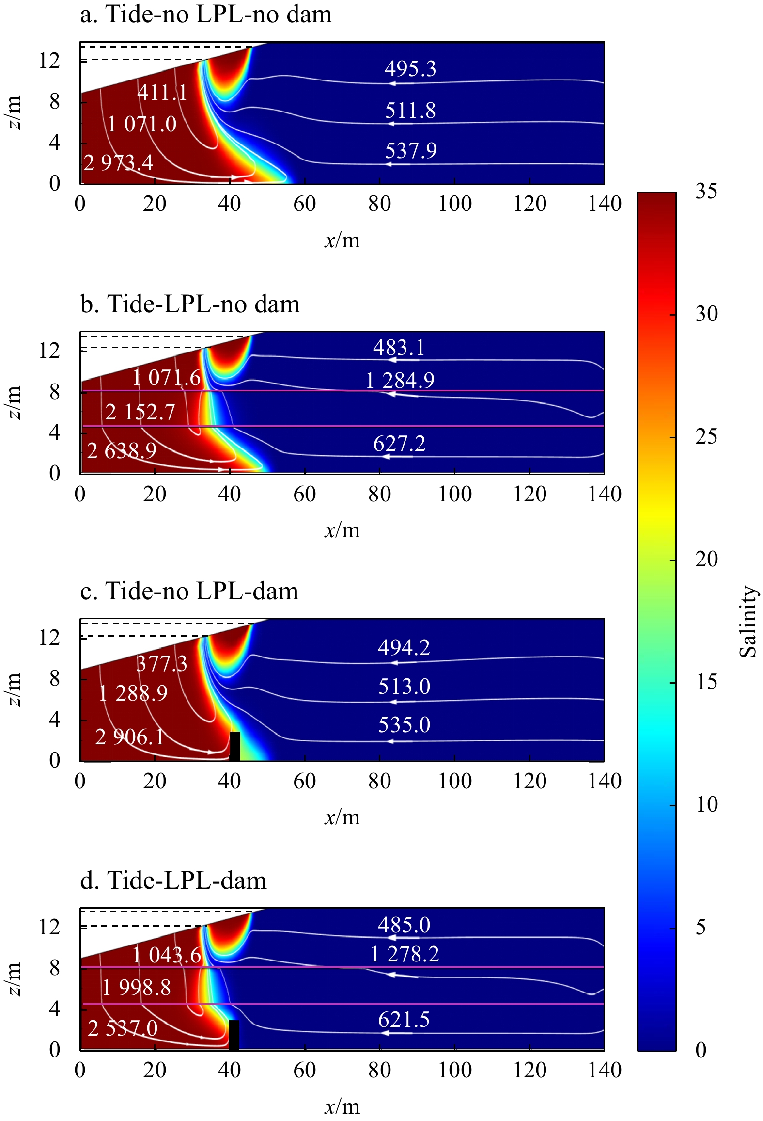
3.2 Salinity distribution

Figure 3 displays color images in a stable state, there are four scenarios: Tide-no LPL-no dam, Tide-LPL-no dam, Tide-no LPL-dam, and Tide-LPL-dam. A freshwater discharge zone separated the circulation cell, and created a USP and SW within the intertidal zone, this USP appeared between the low and high tidal marks. These are consistent with the results of Section 3.1 and previous studies (Fang et al., 2021a; Shen et al., 2020). In the model with an LPL (Fig. 3b), the distribution of the USP and SW are significantly altered compared to the base model without an LPL. As shown in Fig. 3b, the LPL leads to refraction of the boundary between the low and high permeability geological strata. In addition, rising pore water streamlines cause the separation of streamlines of the mixture due to a decrease in pore water flow velocity and result in the formation of a large mixing zone in the LPL, limiting USP extension in the vertical direction. In addition, this moved the SW significantly seaward and showed that stratified aquifers containing an LPL inhibited the invasion of saltwater, i.e., Toe changed from 51.5 m to 47 m, being retreated by 8.7%. Our numerical findings are consistent with field observations of saltwater intrusion in a layered coastal aquifer in Oahu, Hawaii, USA (Oki et al., 1998) and consistent with the experimental and numerical results of Lu et al. (2013).

Figure  3.  Variations in salinity distribution and particle trajectories within the aquifer under different scenarios. The trajectories and time of the particles (beginning at the land boundary and the shoreline) are indicated (in days). The horizontal black dash line indicates the tidal range and the vertical black rectangle indicates the subsurface dams. The horizontal pink line indicates the interfaces of low-permeability layer (LPL). x and z are the horizontal and vertical coordinate values, respectively.

DownLoad: Full-Size Img PowerPoint

Figures 3c and d illustrate the extent of saltwater intrusion under two scenarios: Tide-no LPL-dam and Tide-LPL-dam. In both cases, a subsurface dam was constructed at x = 40 m with a height of 2.6 m, matching the original SW height (the vertical distance between the 50% salinity contour and the x-axis). The presence of subsurface dams significantly alters salinity distributions. In the scenario without an LPL, the dam height of 2.6 m proved inadequate, the natural removal of residual saltwater could not be completed successfully. Consequently, low-salinity saltwater overflowed the dam crest and infiltrated the inland areas 1800 days following the subsurface dam’s construction (Fig. 3c). In contrast, with an LPL present, the mixing zone widened near the dam in the landward aquifer after 442 d but residual saltwater was successfully flushed out. This demonstrates that an LPL can increase the effectiveness of subsurface dams for saltwater intrusion management. The same dam design improves resilience to saltwater intrusion compared to the situation without the LPL (Figs 3c, d).

3.3 Groundwater flow and circulation

In aquifer systems with an LPL, upwardly circulating saltwater undergoes refraction when passing between the lower and upper permeable strata (Lu et al., 2013; Rumer and Shiau, 1968). According to the refraction law (Bear, 1972), at the interface between layers, the refracted angle is less than the injection angle if flowing into the lower permeability layer. This causes an increase in the refracted pore water flowlines within the LPL (Figs 3a-d). Conversely, if flowing into the higher permeability layer, the refracted angle is greater than the injection angle at the interface. This decreases the refracted pore water flowlines in the more permeable stratum. Both the refracted flowlines and the presence of the LPL act to restrict the vertical extension of the water table (Figs 3a, b).

To elucidate the impact of LPL and dam on groundwater flow and saltwater circulation, we conducted a detailed quantitative analysis on the particle travel time (please refer to Xin et al. (2010) for the averaged values during the tidal cycle to see details) (see Fig. 3). We deployed three particles to both the inland boundary and the shore surface, correspondingly (refer to Table 1 for the initial position). Under the Tide-no LPL-no dam case (Fig. 3a), particles released from inland along the moving path of freshwater bypass the USP and SW discharge to the sea. Particles at greater depths required more time compared to those at shallower, e.g., the particle starting from a shallow location (x = 140 m, z = 10 m) took 495.3 d, whereas the particle starting from a deeper inland location (x = 140 m, z = 2 m) took 537.9 d (Fig. 3a, Table 1), increased 8.6%. At the beach surface, the particles released to the deeper beach moved further landward and took longer paths. In this way, the travel time of deeper beach was longer, e.g., the one starting from x = 25 m, z = 11.5 m took 411.1 d, while from x = 5 m, z = 9.5 m took 2 973.4 d (Fig. 3a), increased 623.3%. With the LPL at present (Fig. 3b), the LPL limited the USP extension vertically and modified the travel time of the particles, leading to the pore water refraction occurs in the two layers between the LPL and the high-permeability layer (HPL), e.g., the one starting from the shallow (x = 140 m, z = 10 m) took 483.1 d, while from the deep inland (x = 140 m, z = 2 m) took 627.2 d (Fig. 3b), the one starting from the LPL (x = 140 m, z = 6 m) took 1 284.9 d, increased 151% compared with no LPL action (511.8 d). The SW was moved towards the sea due to LPL activity, which in turn affected the time it took for particles to reach the shore, e.g., a particle released from x = 25 m, z = 11.5 m took 1 071.6 d (Fig. 3b), increased 160.7% compared with no LPL action (411.1 d) (Fig. 3a).

The presence of subsurface dams in the aquifer caused significant alterations to both the particle movement path and travel time (Figs 3c, d in comparison with Figs 3a, b). Particles emitted from the far-reaching inland area began to circumvent the dam by ascending. In this way, travel time was significantly modified in the presence of the dam, e.g., under the dam at x = 40 m, the one starting from x = 140 m and z = 2 m took 535 d (Fig. 3c, Table 1). As the subsurface dams blocked the movement of saltwater, resulting in a reduction in both the path and time of particle travel along the coast, e.g., particles released from x = 25 m, z = 11.5 m (Fig. 3c) took 377.3 d to reach their destination, decreased 9%. In the presence of the dam and LPL, the LPL in the aquifer behaved similarly to the dam, blocking the movement of saltwater into the freshwater zone and preventing USP extension. There were notable alterations in both particle movement and travel time. Superficial particles circumvented the lower USP before being released into the ocean. The travel time related to it reduced, for example, the particle starting from x = 140 m and z = 6 m required 1 278.2 d. Conversely, deep particles bypassed the dam, resulting in an increase in travel time. For instance, the particle starting from x = 140 m and z = 2 m took 621.5 d, compared to 627.2 d in the aquifer without the dam. The travel time for particles passing through the saltwater region decreased due to the hindrance of the dam on the SW movement, as indicated in LPL (Fig. 3b in comparison with Fig. 3d), e.g., the one starting from x = 25 m, z = 11.5 m took 1 043.6 d, it decreased 2.6% contrast with the Tide-LPL-no dam case (1 071.6 d). The findings indicate that the combination of underground barriers and LPLs has an impact on the movement and distribution of groundwater in unconfined aquifers.

3.4 Sensitivity analysis

3.4.1   Sensitivity analysis on the penetration height of subsurface dam

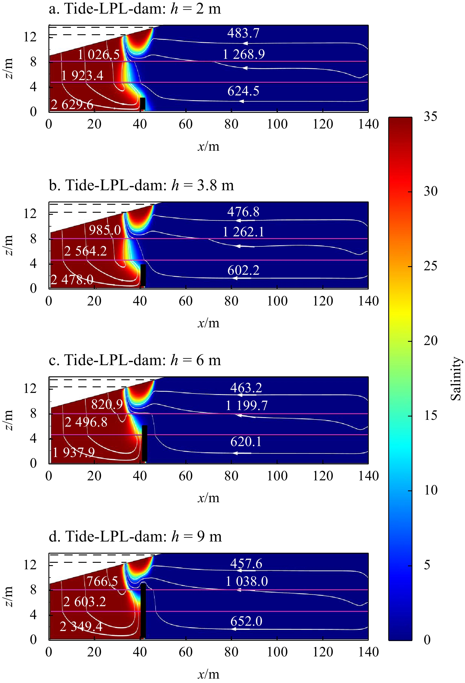
The salinity distribution and groundwater flow are depicted in Fig. 4, showing the influence of subsurface dam height. As anticipated, higher dams more effectively inhibited saltwater intrusion, and the salt content increased to the left of the dam with greater heights. Higher dams also restricted the downward movement of the USP to a greater extent.

Figure  4.  Variations in salinity distribution and particle trajectories within the aquifer under different dam height. The trajectories and time of the particles (beginning at the land boundary and the shoreline) are indicated (in days). The horizontal black dash line indicates the tidal range and the vertical black rectangle indicates the subsurface dams. The horizontal pink line indicates the interfaces of low-permeability layer (LPL). x and z are the horizontal and vertical coordinate values, respectively.

DownLoad: Full-Size Img PowerPoint

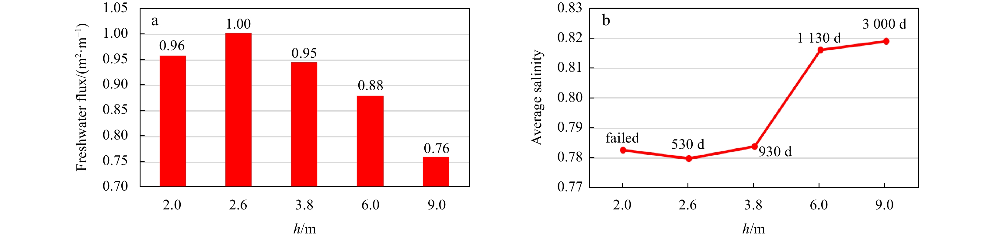
To investigate the effect of barrier height on saltwater intrusion and freshwater discharge, we calculated the average salinity and freshwater discharge in the aquifer per unit width. The freshwater discharge and salinity distribution significantly changed, the salinity increase with the dam height, e.g., when the height was increased to 9 m and salinity increased to 0.818. The freshwater flux increases and then decreases with increasing the height of subsurface dam, e.g., when the dam height was 2 m, and freshwater discharge was 0.96 m²/m, when the dam height was 2.6 m, and freshwater discharge was 1.0 m²/m, when the height was increased to 9 m and freshwater discharge decreased to 0.76 m²/m (Fig. 5a). This is because when the dam heights are below the minimum effective dam height, after dam construction, freshwater velocity was large in the dam upper (Fang et al., 2023). This led to the freshwater discharge increasing with dam heights, and freshwater discharge peaked at the effective dam height. As the dam height exceeds the effective dam height, the discharge tubes of freshwater are squeezed by the dam (Fang et al., 2021b). This leads to the freshwater discharge decreasing with dam heights. In addition, we calculated the time (t_r) required for the natural removal of residual saltwater after installation of the subsurface dams, and the time (t_r) required for natural removal increased with dam height, e.g., the time (t_r) of the natural removal of residual saltwater from 530 d to 3 000 d as the dam height from 2.6 m to 9 m. For a dam height of 2 m, low salinity brackish water exceeds the top of the dam, which is able to continuously replenish the residual saline water behind the dam, making it impossible for the dam to control saltwater intrusion under these conditions.

Figure  5.  Freshwater discharge (a) and average salinity (b) after the construction of subsurface dams under different dam height. In b, the black data are the time natural removal of residual saltwater (unit: d).

DownLoad: Full-Size Img PowerPoint

To interpret the reason why the barrier height impacts saltwater intrusion and freshwater discharge, we conducted a detailed quantitative analysis on the particle travel time (Fig. 4). We deployed three particles to both the inland boundary and the shore surface, correspondingly (refer to Table 2 for the initial position). Particles released from inland experience longer travel times as the dam height increases, this is due to the longer time bypassed the dam, e.g., the particle released from x = 140 m and z = 2 m is 602.2 d of 3.8 m dam height, and travel time is 652 d at h = 9 m, increase 8.3%.

Table  2.  Particle travel times and starting position

Starting position	Particle travel time
	h = 2.0 m	h = 3.8 m	h = 6.0 m	h = 9.0 m
x = 5 m, z = 9.5 m	2 629.6 d	2 478.0 d	1 937.9 d	2 349.4 d
x = 15 m, z = 10.5 m	1 923.4 d	2 564.2 d	2 496.8 d	2 603.2 d
x = 25 m, z = 11.5 m	1 026.5 d	985.0 d	820.9 d	766.5 d
x = 140 m, z = 2 m	624.5 d	602.2 d	620.1 d	652.0 d
x = 140 m, z = 6 m	1 268.9 d	1 262.1 d	1 199.7 d	1 038.0 d
x = 140 m, z = 10 m	483.7 d	476.8 d	463.2 d	457.6 d
Note: h is the dam height; x and z are the horizontal and vertical coordinate values, respectively.

 | Show Table

DownLoad: CSV

3.4.2   Sensitivity analysis on the location of subsurface dam

The impact of the location of a subsurface dam on the effectiveness of managing saltwater intrusion and freshwater discharge was investigated in the presence of an LPL. For the first trial, the dam height was set to 2.6 m at different locations (x = 36 m, x = 38 m, x = 42 m, and x = 44 m). At x = 36 m and 38 m, the removal of residual saltwater could not be completed successfully; therefore, we changed the dam height to control saltwater intrusion.

Figure 6 shows the effect of subsurface dam location on salinity distribution and freshwater flow. As expected, dams positioned farther seaward required greater optimal heights to effectively limit saltwater intrusion, shown through a more landward placement of the saltwater toe.

Figure  6.  Variations in salinity distribution and particle trajectories within the aquifer under different dam location. The trajectories and time of the particles (beginning at the land boundary and the shoreline) are indicated (in days). The horizontal black dash line indicates the tidal range and the vertical black rectangle indicates the subsurface dams. The horizontal pink line indicates the interfaces of low-permeability layer (LPL). x and z are the horizontal and vertical coordinate values, respectively.

DownLoad: Full-Size Img PowerPoint

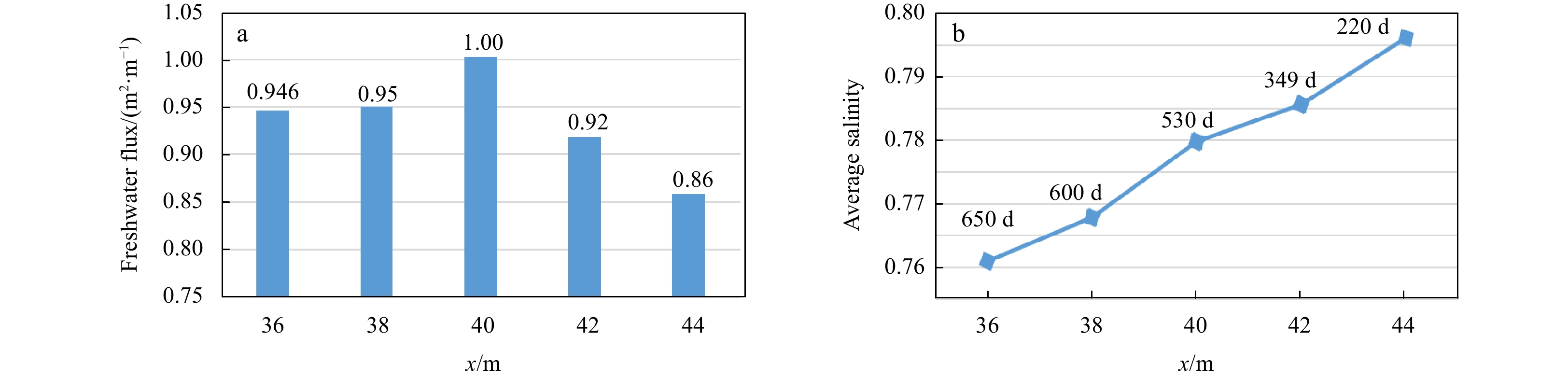
To investigate the effect of the barrier location on saltwater intrusion and freshwater discharge, we calculated the average salinity and freshwater discharge per unit width of the aquifer (Fig. 7). The salinity distribution significantly changed, and it rises as the distance between the dam location and the ocean boundary increases, e.g., when the dam at x = 36 m, the salinity was 0.76, when the dam was moved to x = 42 m, salinity changed to 0.786 (Figs 7a, b). The rise of the upstream water table increases gradually as the distance from the dam location decreases (Fang et al., 2021b), resulting in an increase in freshwater, e.g., when the dam from at x = 36 m moved to x = 40 m, the freshwater discharge from 0.946 m²/m increase to 1.000 m²/m. As the dam height exceeds the effective dam height, causing the dam to compress the discharge tubes of freshwater (Fang et al., 2021b). However, as dams are positioned farther seaward, the degree of constraint on freshwater flow lessens gradually. Consequently, freshwater discharge increases with decreasing distance between the dam location and the ocean boundary, as flow constriction is decreased, e.g., when the dam was moved to x = 44 m, the amount of freshwater decreased to 0.86 m²/m. In addition, we calculated the natural removal time after installation of the subsurface dams, and t_r decreased with distance from the dam location to the sea boundary.

Figure  7.  Freshwater discharge and average salinity after the construction of subsurface dams under different dam location. In b, the black data are the time natural removal of residual saltwater.

DownLoad: Full-Size Img PowerPoint

To interpret the barrier location impacts on saltwater intrusion and freshwater discharge, we conducted a detailed quantitative analysis on the particle travel time (Fig. 6). We deployed three particles to both the inland boundary and the shore surface, correspondingly (Table 3). The time of travel for particles released from the inland deeper extends as the distance from the dam location to the sea boundary increases, e.g., the particle released from x = 140 m and z = 2 m is 592.2 d of the dam at x = 38 m, and travel time is 608.2 d of the dam at x = 44 m, increased 2.7%.

Table  3.  Particle travel times and starting position

Starting position	Particle travel time
	Dam position x = 36 m	Dam position x = 38 m	Dam position x = 42 m	Dam position x = 44 m
x = 5 m, z = 9.5 m	2 518.4 d	2 557.9 d	2 599.6 d	2 595.4 d
x = 15 m, z = 10.5 m	1 665.9 d	1 633.1 d	2 042.7 d	2 168.3 d
x = 25 m, z = 11.5 m	1 081.0 d	1 033.5 d	1 046.8 d	1 050.9 d
x = 140 m, z = 2 m	607.1 d	592.2 d	601.7 d	608.2 d
x = 140 m, z = 6 m	1 256.9 d	1 251.7 d	1 268.3 d	1 272.1 d
x = 140 m, z = 10 m	479.0 d	478.0 d	478.1 d	478.6 d
Note: x and z are the horizontal and vertical coordinate values, respectively.

 | Show Table

DownLoad: CSV

These results suggest that dam location affects freshwater flow and saltwater intrusion in stratified coastal aquifers. Specifically, as the height of the dam surpasses the effective dam height and the discharge of freshwater rises as the distance between the dam location and the ocean boundary decreases, the time (t_r) for the natural removal of residual saltwater extends.

3.4.3   Sensitivity to LPL

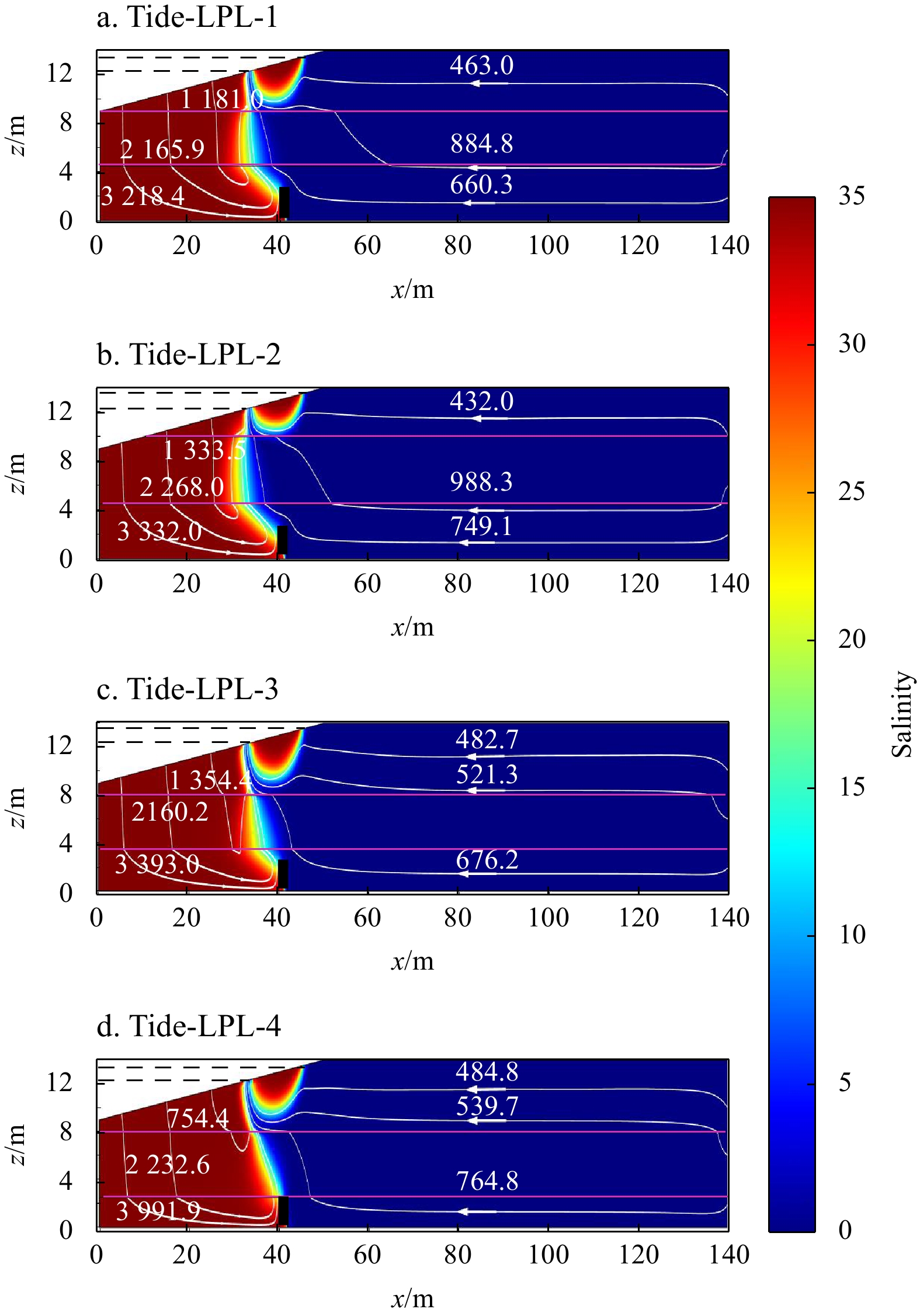
This section explored the impact of the LPL on the effectiveness of managing saltwater intrusion and freshwater discharge when a dam is present. To investigate the impact of various LPLs using a constant dam height of 2.6 m (we define the upper boundary and bottom boundary of LPL are z₁ and z₂, respectively, we considered four cases as follows: LPL-1 case: z₁ = 9 m, z₂ = 4.5 m; LPL-2 case: z₁ = 10 m, z₂ = 4.5 m; LPL-3 case: z₁ = 8 m, z₂ = 3.5 m; and LPL-4 case: z₁ = 8 m, z₂ = 2.5 m).

Figure 8 shows the effect of the LPL on salinity distribution and freshwater flow. USP compression gradually occurred as the upper boundary (z₁) of the LPL became shallower, while the area of the mixing zone increased. In contrast, although the USP moved deeper as the bottom boundary (z₂) of the LPL, but the SW moved inland significantly and rose obviously under the left of the dams, leading to a decrease in the area of the mixing zone.

Figure  8.  Variations in salinity distribution and particle trajectories within the aquifer under different low-permeability layer (LPL). The trajectories and time of the particles (beginning at the land boundary and the shoreline) are indicated (in days). The horizontal black dash line indicates the tidal range and the vertical black rectangle indicates the subsurface dams. The horizontal pink line indicates the interfaces of LPL. x and z are the horizontal and vertical coordinate values, respectively.

DownLoad: Full-Size Img PowerPoint

We calculated the average salinity and freshwater discharge in the aquifer per unit width (Fig. 9). The freshwater discharge and salinity distribution significantly changed. As the upper boundary of the LPL moves towards shallower layers and the SW retreats, the dam height exceeds the minimum effective dam height, so the freshwater discharge and the average salinity decrease as the upper boundary moves toward shallower layers, e.g., when the upper boundary (z₁) at 8 m, the freshwater discharge was 1.0 m²/m, and salinity was 0.78, when the upper boundary (z₁) at 10 m, the amount of freshwater decreased to 0.52 m²/m, and salinity changed to 0.72 (Figs 9a, b). As the bottom boundary moves towards deeper layers, SW further intrudes into the inland and leads to the average salinity increased (Figs 8 and 9b). Meanwhile, the difference between the dam height and the minimum effective dam height decreased, thus the freshwater discharge increases (Figs 8 and 9a). However, when the bottom boundary at z = 2.5 m, the impact of the dam on the freshwater discharge is no longer significant, so the freshwater discharge decreases with the further intrusion of SW (Figs 8 and 9a). Furthermore, we conducted calculations of the time (t_r) necessary for the natural removal of residual saltwater following the implementation of subsurface dams. The results revealed that the time (t_r) required for natural removal decreased when the upper boundary (z₁) of the LPL was moved to shallower regions. Conversely, when the bottom boundary (z₂) of the LPL was moved to deeper regions, the time (t_r) increased, e.g., the time (t_r) of the natural removal decreased from 530 d to 148 d as the z₁ from 8 m to 10 m and increased to 551 d as the z₂ moved to 2.5 m. Three particles were introduced at the inland boundary and the beach surface (Table 4). The time of travel for the particles emitted from the inland deeper extended as the LPL thickness increased, e.g., the particle released from x = 140 m and z = 2 m is 749.1 d for z₁ at 10 m (Fig. 8b), and travel time is 621.5 d at z₁ = 8 m (Fig. 3d), and released from the sea beach increase with the thickness of LPL, e.g., the particle released from x = 5 m, z = 9.5 m is 3 332 d of z₁ at 10 m (Fig. 8b), and travel time is 2 537 d at z₁ = 8 m (Fig. 3d).

Figure  9.  Freshwater discharge and average salinity after the construction of subsurface dams under different low-permeability layer. In b, the black data are the time natural removal of residual saltwater.

DownLoad: Full-Size Img PowerPoint

Table  4.  Particle travel times and starting position

Starting position	Particle travel time
	z1 = 9 m, z2 = 4.5 m	z1 = 10 m, z2 = 4.5 m	z1 = 8 m, z2 = 3.5 m	z1= 8 m, z2 = 2.5 m
x = 5 m, z = 9.5 m	3218.4 d	3332 d	3393 d	3991.9 d
x = 15 m, z = 10.5 m	2165.9 d	2268 d	2160.2 d	2232.6 d
x = 25 m, z = 11.5 m	1181 d	1333.5 d	1354.4 d	754.4 d
x = 140 m, z = 2 m	660.3 d	749.1 d	676.2 d	764.8 d
x = 140 m, z = 6 m	884.8 d	988.3 d	521.3 d	539.7 d
x = 140 m, z = 10 m	463 d	432 d	482.7 d	484.8 d
Note: x and z are the horizontal and vertical coordinate values, respectively; z1 and z2 are the upper and bottom boundaries of the LPL.

 | Show Table

DownLoad: CSV

These results suggest that the LPL affects salinity distribution, freshwater flow and effective dam control of saltwater intrusion in stratified coastal aquifers. In greater detail, the relocation of the upper boundary (z₁) of the LPL to shallower regions resulted in significant changes. The USP contracted, the mixing zone area expanded, and the time (t_r) needed for the natural removal of residual saltwater decreased considerably. As the bottom boundary (z₂) of the LPL was relocated to deeper regions, the mixing zone area decreased, consequently increasing the risk of inadequate subsurface dam control over saltwater intrusion.

4. Discussion

Most previous studies investigated the individual effects of subsurface dams and tides on aquifer stratification, and revealed that subsurface dams control saltwater intrusion. However, there has been little research on the combined impact of LPL and tidal on subsurface dam control of saltwater intrusion. As evident from the LPL cases simulated here, a more complex problem to consider is whether subsurface dams can control saltwater intrusion.

These results revealed how the LPL impacts the effectiveness of subsurface dams concerning salinity distribution and freshwater flow. When the upper boundary of the LPL moves towards shallower layers, the USP contracts, and the area of the mixing zone increases due to the low K of clay. Since the SW moved seaward slightly, and we could appropriately reduce the height of the dam. As the bottom boundary of the LPL was moved to deeper regions, the refracted pore water streamlines in the LPL moved inland, moving the salt-freshwater interface away from the ocean. Most importantly, the area of the mixing zone decreased or increased the risk of poor subsurface dam control of saltwater intrusion, so we chose a greater dam height.

The gradual attention towards the removal of residual saltwater following the establishment of underground barriers has been observed (Kang et al., 2021; Ke et al., 2021; Kang and Xu, 2017). Some previous studies reported that residual saltwater remains trapped in upstream aquifers for decades (Zheng et al., 2021), affecting the availability of freshwater. Present study revealed the time required for natural purification increases with the dam height increases. Interestingly, the natural removal time was much less than previously reported, e.g., the time (t_r) required for the removal time of residual saltwater increased to 3 000 d at a dam depth of 9 m. This is almost likely occurred due to tide activity and the presence of the LPL. For example, Zheng et al. (2021) revealed that for dam heights more than 16 m, residual saltwater removal took more than 50 years and that an increase in dispersivity from 1 m to 3 m dramatically reduces desalinization time from more than 30 years to 4 years, but they considered the hydrostatic boundary. In addition, the LPL impacts the natural residual saltwater. As shown in Fig. 9b, the time required for the natural removal of residual saltwater decreased significantly as the upper boundary LPL was moved to shallower regions.

It should be noted that the aquifer for which this study primarily concerned is a stratified geologic structure. However, layered aquifers are just one type of geologic heterogeneity, another important heterogeneity is spatially random heterogeneity (Kreyns et al., 2020), and this more complex saltwater intrusion process should be considered in future work. In addition, the inland boundary condition was head specified, while as a sinusoidal tide was considered at the seaside boundary. Actually, the inland freshwater flux may fluctuate seasonally, the tidal cycles may be longer (e.g., spring-neap tides) and more complex seaside boundaries (e.g., waves and storm surges), should be carefully considered in practical applications.

5. Conclusions

In this study, we numerically examined the combined effect of subsurface dams and a typical stratified aquifer (two HPLs with an LPL between them) on groundwater flow and salinity distribution in a tidally influenced coastal unconfined aquifer. Additional problems encountered after the construction of subsurface dams were also evaluated using the following indexes: freshwater discharge, average salinity, and the time (t_r) required for the natural removal of residual saltwater. The key findings are as follows.

(1) In stratified coastal aquifers LPL can increase the effect of subsurface dams to control saltwater intrusion.

(2) The combination of tides and LPL remarkably influence the salinity distribution and groundwater flow, and enhance the removal rate of natural residual saltwater.

(3) When the upper boundary of the LPL moves towards shallower layers, the area of the mixing zone increases, and the USP area and the time required for the natural removal of residual saltwater decrease, and could appropriately reduce the height of the dam.

(4) If the bottom boundary of the LPL is moved to deeper regions, the mixing zone decreases or enhances the risk for poor subsurface dam control of saltwater intrusion. For this reason, higher dam is suggested.