


Figure
1.
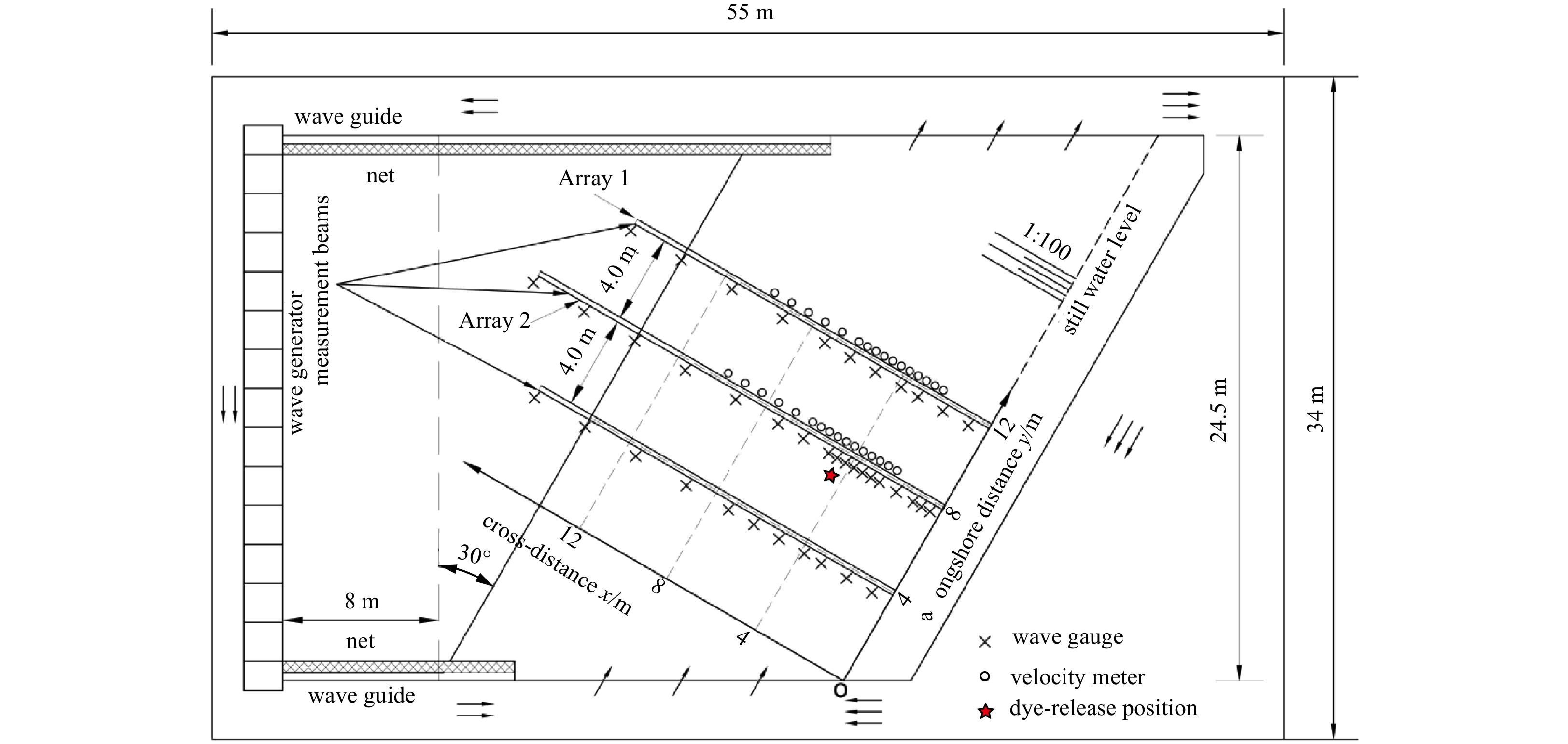
Experimental layout.
| Citation: | Chunping Ren, Nannan Fu, Chong Yu, Yuchuan Bai, Kezhao Fang. Observing eddy dye patches induced by shear instabilities in the surf zone on a plane beach[J]. Acta Oceanologica Sinica, 2024, 43(3): 15-29. doi: 10.1007/s13131-023-2270-y

|
The surf zone extends from the breaker zone to the shore and to the seaward extent of depth-limited breaking, characterized dynamically by the importance of eddies and wave-driven flows. At the shoreline, pollutants can enter through storm overflow discharges from overloaded combined and separate sewerage systems during rainfall events, thus making the surf zone crucial for nearshore ecosystems. Alongshore currents (Feddersen, 1998; Longuet-Higgins, 1970; Tang et al., 2016) are induced under obliquely incident wave conditions in the surf zone when wave breaking occurs. Simultaneously, turbulence (Feddersen, 2012) is generated, so the water column (Hally-Rosendahl et al., 2014) is vertically mixed. Field observations and modeling indicate that surf zone eddies (Clark et al., 2010, 2011; Spydell and Feddersen, 2012a) significantly affect the dispersion and dilution of surf zone pollutants (Clark et al., 2010, 2011; Spydell and Feddersen, 2012a, b) and material transport (e.g., of larvae and nutrients) between the surf zone and inner shelf (Brown et al., 2015; Hally-Rosendahl and Feddersen, 2016; O’Dea et al., 2021; Wu et al., 2020). The generation mechanism of surf zone eddies includes intrinsic shear instability (Noyes et al., 2004; Oltman-Shay et al., 1989) and extrinsic wave forcing (short crested (Feddersen, 2014; Peregrine, 1998) or wave groups (Long and Özkan-Haller, 2009; Reniers et al., 2004)). It was suggested that shear instability might dominate surfzone eddy generation for highly narrowbanded frequency and direction and obliquely large incident waves (Feddersen, 2014). However, the eddies’ evolution of surf zone tracers is poorly understood.
According to linear stability theory, background vorticity
Although Feddersen (2014) suggested that surfzone eddies (vorticity) are generated through the extrinsic mechanism of breaking wave vorticity forcing, with a 10–100 m range alongshore, the modeling snapshot result at t = 91.2 min showed that simulated tracer patch meanders 0–100 m alongshore, utterly different with downstream dye patches (
According to the extrinsic wave-breaking mechanism in generating surf zone eddies, the eddies coalesce to form transient rip currents. The episodic offshore directed flows eject surf zone water onto the inner shelf (Johnson and Pattiaratchi, 2004). Further, the material exchange between the surf zone and inner shelf associated with transient rip currents has been studied using a numerical method and field observations (Grimes et al., 2020a, 2020b, 2021; Hally-Rosendahl et al., 2014, 2015; Moulton et al., 2021; O’Dea et al., 2021). Therefore, these surf zone eddies are critical to the material exchange, and exploring the generation forced by shear instabilities is necessary.
Shoreline dye release experiments in fields have been conducted to quantify the surf zone tracer transport and exchange between the surf zone and inner shelf (Clark et al., 2010; Grimes et al., 2021; Hally-Rosendahl et al., 2014, 2015). Whether these release experiments were continuous or instantaneous, long or short alongshore, these observations show that the maximum tracer concentration occurs roughly periodically alongshore from the release location to the tracer front position. Correspondingly, the tracer head in the cross-shore direction is rhythmic in the surf zone and on the inner shelf.
Alongshore meandering (spreading) tracer patches are commonly ascribed to shear instability or dispersion. According to linear stability theory, the generated shear waves have phase velocities, lengths, and time scales in the alongshore direction. The extrinsic wave-breaking mechanism in generating surfzone eddies cannot sufficiently describe these alongshore current oscillations (Noyes et al., 2005; Oltman-Shay et al., 1989; Ren et al., 2012). However, after dye release, a prolonged surf-zone concentration decay
When the alongshore wave-guide current is generated (due to the shear of the alongshore current in the cross-shore direction), it is yet unverified whether the turbulence caused by the wave breaking is also affected by the shear of the current. This concept has not been studied using models that consider shear instability and wave breaking. For weak alongshore currents or V = 0, the vertical change of the currents in the surf zone is enhanced, resulting in the vertical shear of current enhancements. According to shear instability theory, as long as there is a flow shear, the background vorticity can be generated, driving the generation of these eddies. Therefore, the surf zone vortex observed in the case of a weak current is also very likely to be driven by the current shear force and gradually evolve into a large-scale vortex.
Regarding these eddies caused by the shear instability of the alongshore current, the corresponding tracer experiment and the impact on the propagation and diffusion of pollutants inside and outside the surf zone need further study. The use of pollutants or floats for field or laboratory experiments can efficiently investigate the mixing (Abolfathi and Pearson, 2017; Abolfathi et al., 2020), the propagation of pollutants and eddy generation mechanism in the surf zone, observe the characteristics of the vortex in the surf zone, and verify the mathematical model (Abolfathi and Pearson, 2014; Clark et al., 2011; Grimes et al., 2021; Pearson et al., 2009). The surf zone tracer diffusion and dispersion can be studied by measuring the concentration distribution on the cross-section (Clark et al., 2010), remote sensing (Grimes et al., 2021), radar (O’Dea et al., 2021), and laboratory image (Abolfathi and Pearson, 2014). The first three are more suitable for large-scale analysis in the field, but the accuracy is relatively low. Laboratory image acquisition has advantages in terms of accuracy, and the subtle processes of propagation, diffusion, and vortex generation in the surf zone can be obtained in a smaller area. Instantaneous or continuous release of pollutants in the surf zone has been used to study the propagation and diffusion of pollution inside and outside the surf zone. Still, none of these studies revealed the effect of shear instability on the propagation and diffusion process of pollutants around or within the surf zone.
Therefore, based on the surf zone tracer laboratory experiment, we studied the characteristics of surf zone eddies and propagation driven by the instability of the alongshore current. The paper also verifies whether the fluctuation of the alongshore current can produce eddies in the surf zone on the alongshore uniform slope under monochromatic, unidirectional, and obliquely incident waves with a large incident angle. The research results may provide an implication for understanding surf zone eddy generated by shear instabilities of alongshore currents.
This paper analyzes laboratory surf zone tracer observations on a plane beach to investigate the behavior of plumes generated by the shear instabilities of alongshore currents. Section 2 describes the laboratory experiment, while Section 3 describes the evolution of the eddy patch. The extension and transport of these eddy patches are estimated by tracking. Section 4 reports the shear instability analysis of four cases. Some study limitations, including experimental and numerical analyses are discussed in Section 5. The conclusions are summarized in Section 6.
To observe the surf zone eddy generated by the instabilities of alongshore currents, we conducted an alongshore current and dye release experiment in the laboratory on the plane beach with slope 1:100 under monochromatic, unidirectional, and obliquely incident waves with a 30° incident angle. The 1:100 slope was chosen to induce a wider surf zone and variations in longshore current velocity gradients (i.e., significant front shear and backshear) in the surf zone, which increases the shear instability. Laboratory experiments on the shear instability of longshore currents have been carried out. For instance, Visser (1991) experimented on alongshore currents on plane slopes 1:10 and 1:20. Still, previous experimental results did not indicate the temporal variations of alongshore currents. Measurements of the unstable motion of alongshore currents suggested that instability occurs on a barred beach but not on a non-barred beach (Reniers et al., 1997). Although they observed oscillations for regular and random waves on a barred beach, Reniers et al. (1997) suggested that such observations do not necessarily preclude shear instability on a plane beach. Elsewhere, the lack of detection of shear waves in laboratory experiments has been attributed to the limited length of the wave basin and the damping effect of bottom friction (Putrevu and Svendsen, 1992), (i.e., the viscous damping probably suppresses the shear instability in laboratory experiments). The observations are described elsewhere (Ren et al., 2012) and briefly introduced here. The experiment was carried out in the 55 m × 34 m × 1.0 m wave basin at the State Key Laboratory of Coastal and Offshore Engineering, Dalian University of Technology. The beach makes an angle of 30° to the wave generator, creating a large incident angle and a long beach that allows more room for alongshore current instability to develop. Two concrete plane profiles with 1:40 and 1:100 slopes were constructed (Fig. 1).
The present study analyzed only the measurement results for the 1:100 slope because the surf zone width is sufficient to detect the shear instabilities as much as possible. Putrevu and Svendsen (1992) mentioned that it is appropriate to consider spatial scales corresponding to this topography when discussing possible shear wave instabilities in laboratory measurements. Another reason is that enough horizontal spatial scale can be provided to transport the dye patch, particularly eddy patch separation. Also, it was demonstrated that the entire process of eddy dye patch formation on the 1:100 slope can be observed, not on the 1:40 slope (according to the present observation). The coordinate system used has x as the cross-shore coordinate that increases offshore with the still water line x = 0 m, and y as the alongshore coordinate. The still-water depth over the horizontal bottom was 0.45 m for the 1:40 slope experiments and 0.18 m for the 1:100 slope experiments. A wave generator consisting of individual wave paddles was located at the offshore end of the basin, having a total length of 24.5 m. The paddles were moved in phases. Monochromatic, random, unidirectional, and obliquely incident waves were generated in the experiments. Irregular waves were generated using a JONSWAP spectrum with a peak enhancement factor γ of 2.5. To make alongshore currents recirculate within the wave basin and produce uniform movements, a circulation channel with a 3.0 m width at the two lateral ends and a 1.0 m depth (the same as in the horizontal bottom part of the basin) was introduced around the beach.
A total of 32 two-dimensional velocity meters (VMs) in two identical arrays of 16 (Fig. 1) measured the flow field at a 20 Hz sampling rate. These VMs were set at one-third of the water depth from the bottom, approximately the depth at which depth-averaged alongshore currents occurred. The distance of the VMs from the shoreline for the slope 1:100,
| VM | $x$/m | VM | $x$/m | |
| 1 | 2.0 | 9 | 6.0 | |
| 2 | 2.5 | 10 | 6.5 | |
| 3 | 3.0 | 11 | 7.0 | |
| 4 | 3.5 | 12 | 8.0 | |
| 5 | 4.0 | 13 | 9.0 | |
| 6 | 4.5 | 14 | 10.0 | |
| 7 | 5.0 | 15 | 11.0 | |
| 8 | 5.5 | 16 | 12.0 |
 DownLoad:
CSV
DownLoad:
CSV
Steady and strong alongshore currents can be generated (Ren et al., 2012). Here, four wave conditions (Table 2) were chosen to analyze the surf zone tracer evolution. The surf-zone width and the offshore values
| Case | Incident wave | Slope | D/cm | H/cm | T/s | xb/m | ${L_0}$ | ${\xi _{\text{0}}}$ | ${{{{H_0}} \mathord{\left/ {\vphantom {{{H_0}} L}} \right. } L}_0}$ |
| 1 | regular waves | 1:100 | 18 | 2.7 | 1.5 | 5.2 | 3.51 | 0.11 | 0.01 |
| 2 | irregular waves | 1:100 | 18 | 2.4 | 1.0 | 6.2 | 1.56 | 0.08 | 0.02 |
| 3 | irregular waves | 1:100 | 18 | 3.9 | 1.0 | 9.8 | 1.56 | 0.06 | 0.02 |
| 4 | irregular waves | 1:100 | 18 | 5.0 | 1.5 | 10.2 | 3.51 | 0.08 | 0.01 |
| Note: $D$, still water depth; $H$, mean wave height; $T$, peak period; ${L_0}$ and ${H_0}$, wave length and wave height at the wave maker, respectively; xb, surf-zone width. | |||||||||
DownLoad:
CSV
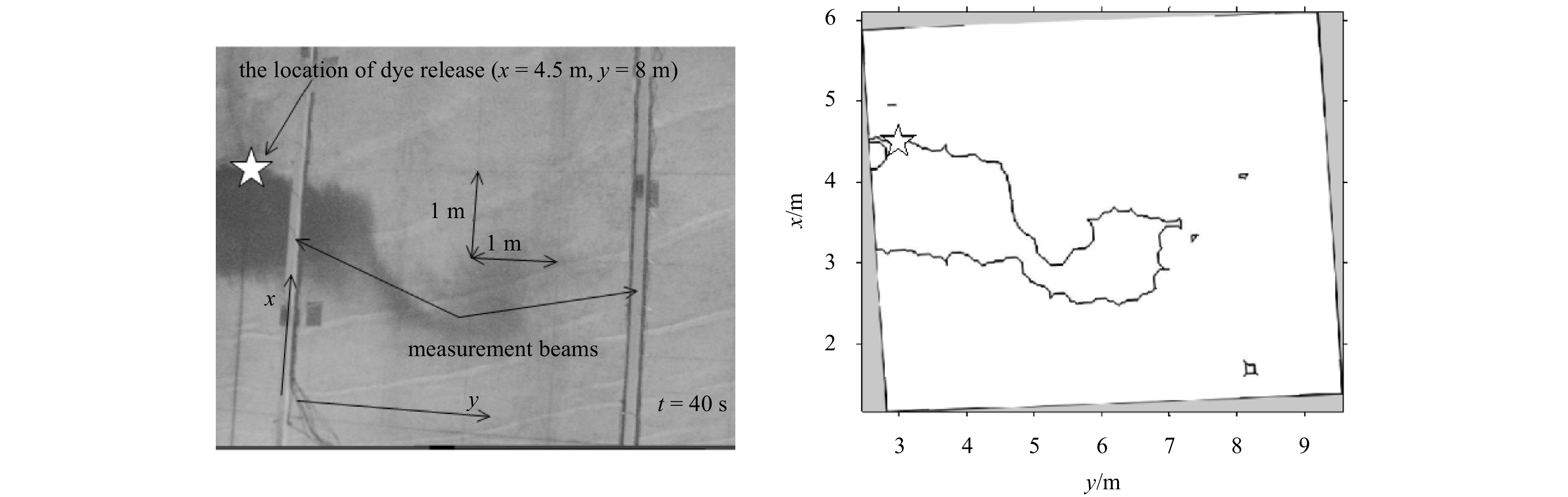
A dye release experiment was conducted to observe the oscillation motions visually and spatially as the longshore currents were generated. The dye (ink, in this case) was continuously released in the surf zone using a long, 0.8 cm-diameter thin tube. The dye-release point was located at

The pixels of the image were 752 × 576, corresponding to 5 m × 7 m (denoting cross-shore and alongshore dimensions, respectively). Figure 2 illustrates the image-collecting system. When the alongshore current was stable (based on the time histories of the current meter), the ink was released continuously into the surf zone simulated by a continuous source. The ink was pulled to the vicinity of the surf zone through a thin tube when released with about 50 cm3/s flow. The CCD system sampled the dye patch movement approximately every 1.0 s until the front part of the dye patch exited the CCD acquisition range under each wave condition.
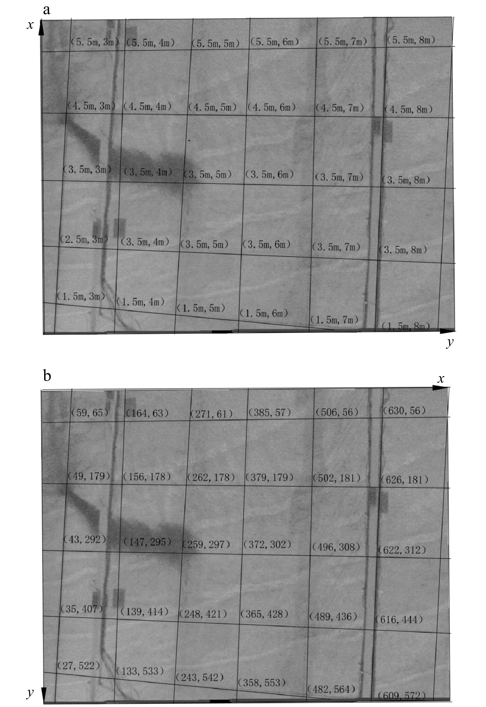
The CCD system collects images with stricter requirements for the brightness of the environment. To collect clear images and coordinate transforms (transforms between world and image coordinates), the beach was made of white cement, forming a white background, and drawn 1 m × 1 m black mesh on the beach, making it easy to accurately analyze the characteristics of the ink patch in the surf zone.
Through experimental analysis, we found that visible eddy or alongshore meandering patches occurred in the four test cases. The parameters are given in Table 1.
The image analysis procedure includes three steps. First, we extracted the dye patch boundaries using the Matlab image processing toolbox. In detail, this step involves subtracting the background image (collected before dye release) from the dye patch image (collected at some time during the dye release experiment), extracting the dye patch boundaries using Matlab image processing toolbox, such as colormap( ), im2bw( ), imclose( ) and so on. Thus, the dye patch boundaries can be obtained with coordinate transform. The second step is coordinate transform. To quantitatively analyze scales and the transport of surf zone dye patches, one necessary requirement for quantifying the information in a dye patch image is knowing the photogrammetric transformation between world and image coordinates. Here, we adopted the coordinate transformation method developed by Holland et al. (1997). These transforms require the world coordinate and the corresponding image coordinate as inputs. The 36 ground control points are used to transform between pixel and world coordinates (Fig. 3). The plane beach in this experiment was painted white, and square grids (1 m × 1 m denotes by two-arrow in Fig. 4 were drawn on the surface to transform from a pixel coordinate into a physical coordinate of identifiable ground control points. Figure 4 shows the image at t = 40 s for Case 1 (left), and the dye patch boundary transformed from pixel coordinate into the physical coordinate. At last, we focus on the eddy dye patches (solid blue rectangular box in Fig. 9), used to quantitatively analyze the diffusion and transport of the eddy patch with time.


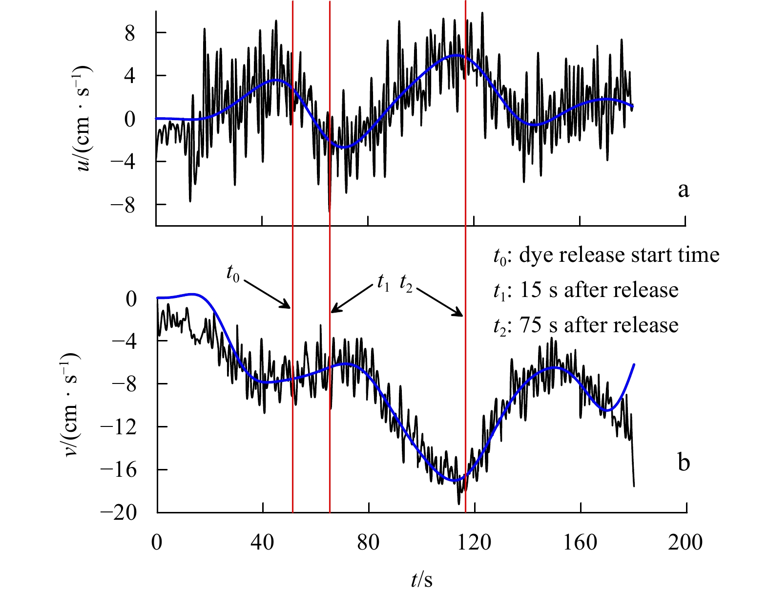
Figure 5 shows the recorded time series of cross-shore and alongshore current velocities for Case 1 (regular waves) at x = 4.5 m in the first velocity meter array. Large-amplitude and long-period oscillations occurred in the alongshore and cross-shore velocity components, also observed under all four conditions, with a 50 s period. The maximum alongshore current velocity (0.18 m/s) present at t = 115 s, and the mean over 40 s (the alongshore currents were gradually strong) to 180 s was approximately 0.12 m/s (Fig. 5b). The cross-shore velocity oscillated between 0.08 m/s and –0.08 m/s (Fig. 5a). To show the far infragravity motions clearly, low-pass finite impulse response filter was then applied to the data with threshold frequencies of 0.02 Hz for irregular waves and 0.04 Hz for regular waves (Fig. 5).

Ren et al. (2012) compared the cross-shore profiles of the mean alongshore velocities for the two velocity meter arrays, demonstrating that the generated mean alongshore currents were approximately uniform. Figure 6 shows the alongshore currents for Cases 1–4 (in meters) deployed in the second velocity meter array close to the dye release location. Each test was repeated thrice throughout the experiment to obtain compelling results; therefore, every cross-shore location had three values (some data were broken).

The longshore current profiles for the four cases (Fig. 6) were computed from the depth-averaged longshore momentum balance (Reniers and Battjes, 1997). The solid curves fitted to the longshore currents velocity measurement are also given. By comparison, we observed that the model results did not match the fitted data adequately, particularly at the shoreward side (frontshear) or seaward side (backshear) of the velocity profile (Baquerizo et al., 2001). Such is attributable to the model parameters. Nevertheless, the fitted results agreed more with the measurements. Based on linear instability theory, the instability mode is sensitive to the mean longshore current profile (Baquerizo et al., 2001). Therefore, the solid curves fitted to the results were used as input data for the linear instability analysis in Section 4. The maximum mean alongshore currents (
By observing the tracer images collected in the experiment, we found that surf zone eddies appeared under all four test conditions, and these tracer eddies gradually developed over time. During this process, these dye patches were meandering in the alongshore direction, similar to the HB06 modeling result at t = 91.2 min downstream of dye release from 0 m to 100 m (
Figure 7 shows the collected images of the dye patch at t = 15 s, 25 s, 35 s, 45 s, 55 s, 65 s, 75 s, 85 s, 95 s, and 105 s for Case 1 in the surf zone. Here, the detailed process of surf zone eddy generation was apparent. At the initial stage t = 15 s (corresponding to t1 indicated using red line in Fig. 5, 15 s since ink release), the alongshore current velocity was about 0.08 m/s, and the ink patch was only transported in cross-shore direction, indicating that the stokes drift at the release position was larger than the alongshore current velocities. When the dye patch was transported onshore at some location, the dye patch gradually moved in alongshore direction due to the considerable increase of alongshore current at this location. Simultaneously, curl deformation occurred because the shear force


In Fig. 8, the collected images for Cases 2–4 under regular incident waves are shown to examine the effects of wave conditions on the deformation pattern of the dye patch. We observed that these dye patches moved meanderingly in Case 2. Significant deformation of these dye patches occurred, and the front part of the dye patch formed an eddy shape. It was ejected offshore and shoreward for Cases 3 and 4, respectively (the solid red rectangular box in Figs 7b and c). In detail, these eddy shape patches for Case 4 were presented more sufficiently and completely than for Case 3. For Case 2, eddy shape patches were not observed, maybe due to the limited collection area. It means that the deformation may occur at some location downstream or in the observation area after a long release time. The above observation for Cases 1–4 demonstrated two types of deformation: meandering and eddy shape. More importantly, the two deformations were continuous; therefore, a persistent driving force was required.

As mentioned in Section 3.1, alongshore currents were strong for the four cases, and the alongshore current shear may be large enough to induce shear instability. Therefore, it suggests that the deformations of these dye patches were dominated by shear instability. For Cases 3 and 4, surf zone eddy shape patches appeared in the offshore and the onshore direction, respectively, indicating that the eddy induced by shear instability may eject shoreward or offshore. The ejection offshore was similar to transient rip currents, characterized by concentrated and ephemeral offshore flows that trap and advect surfzone tracers onto the innershelf, resulting in an alongshore patchy innershelf tracer field (Grimes et al., 2021; Hally-Rosendahl et al., 2014). Based on the previous study, transient rip currents are generated randomly on uniform beaches (Hally-Rosendahl et al., 2015). However, the perturbation velocity field induced by shear instability was periodic in the alongshore direction. That means surf zone eddies generated by shear instability are not random. At least, the meandering dye patch formation cannot be explained using the transient rip current generation mechanism.
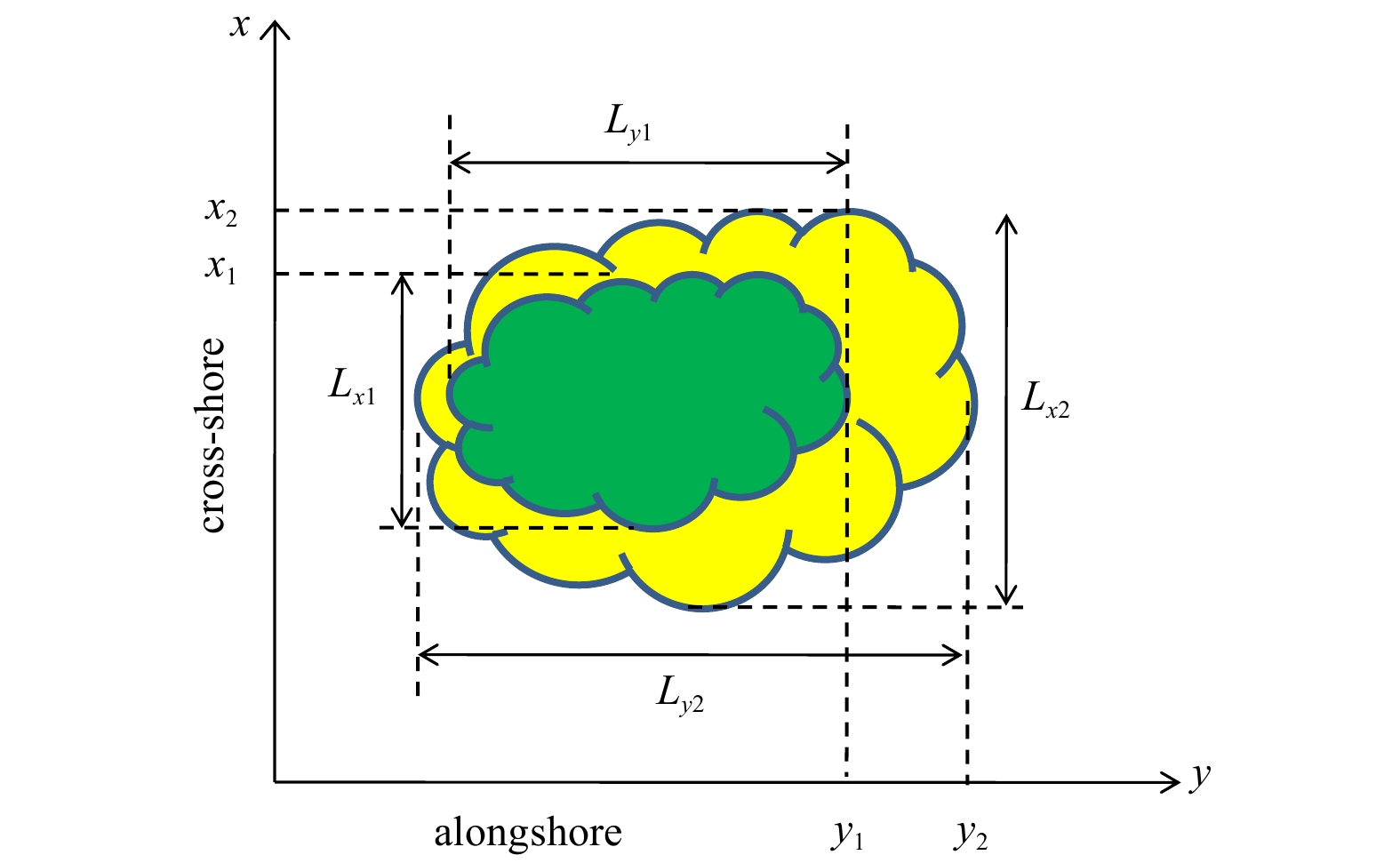
These surf zone eddies significantly impact the diffusion and transport of dye patches in the cross-shore and alongshore direction. Here, quantitative analysis of the diffusion and transport was conducted by tracking the deformation and displacement of the approximate centroid of the eddy patch (the solid blue rectangular box in Fig. 9) with time.
First, these collected images were processed to obtain their boundaries at which the concentration was regarded as approximately 5% of the maximum (Figs 3 and 8). Next, we examined the diffusion and transport of eddy patches.
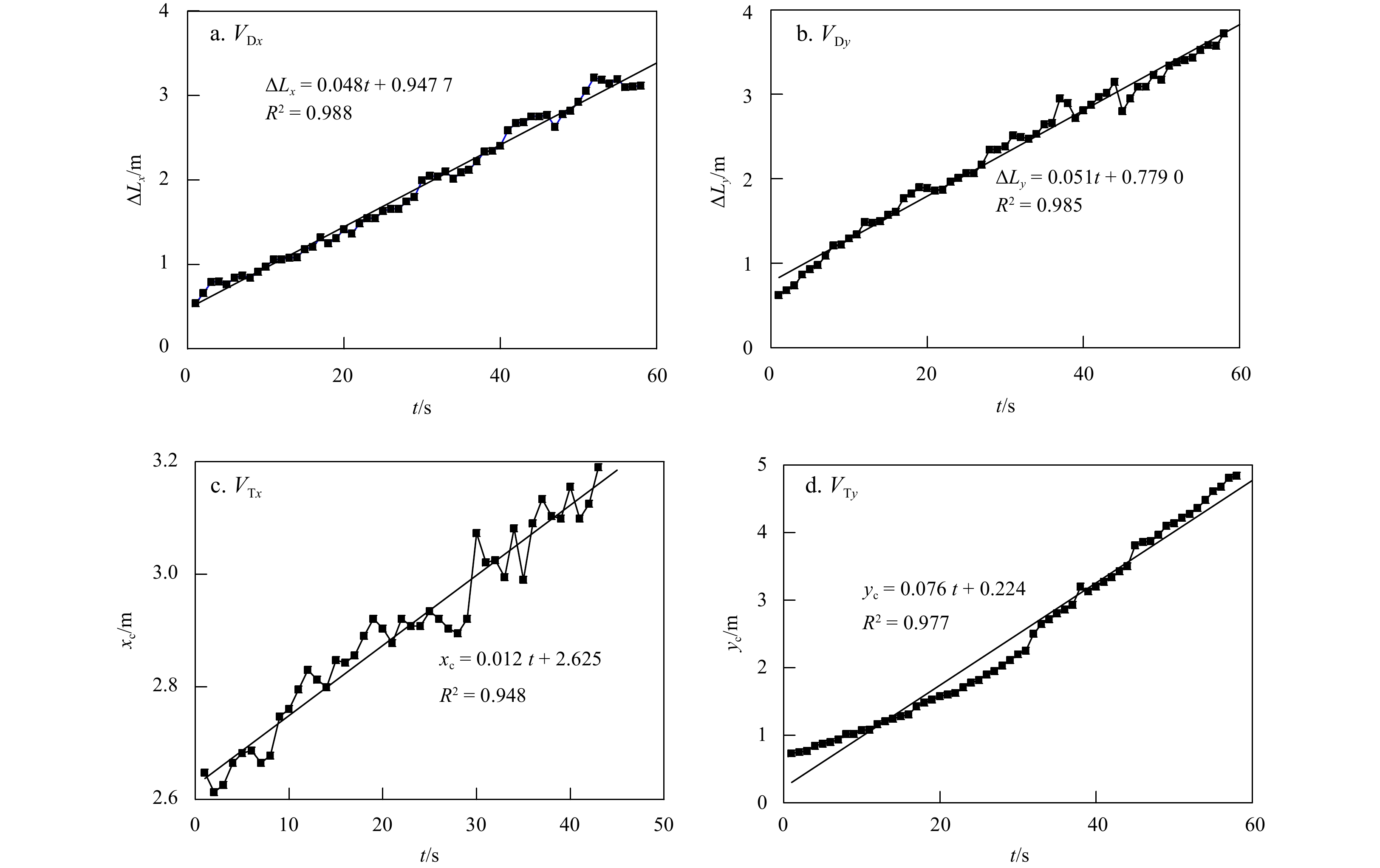
Here, diffusion velocities (

| $$ {V_{{\rm D}x}} = \frac{{\Delta {L_x}}}{{\Delta t}} , $$ | (1) |
| $$ {V_{{\rm D}y}} = \frac{{\Delta {L_y}}}{{\Delta t}} , $$ | (2) |
| $$ {V_{{\rm T}x}} = \frac{{\Delta {S_x}}}{{\Delta t}} , $$ | (3) |
| $$ {V_{{\rm T}y}} = \frac{{\Delta {S_y}}}{{\Delta t}} , $$ | (4) |
where
Based on the definition of diffusion and transport velocity given,
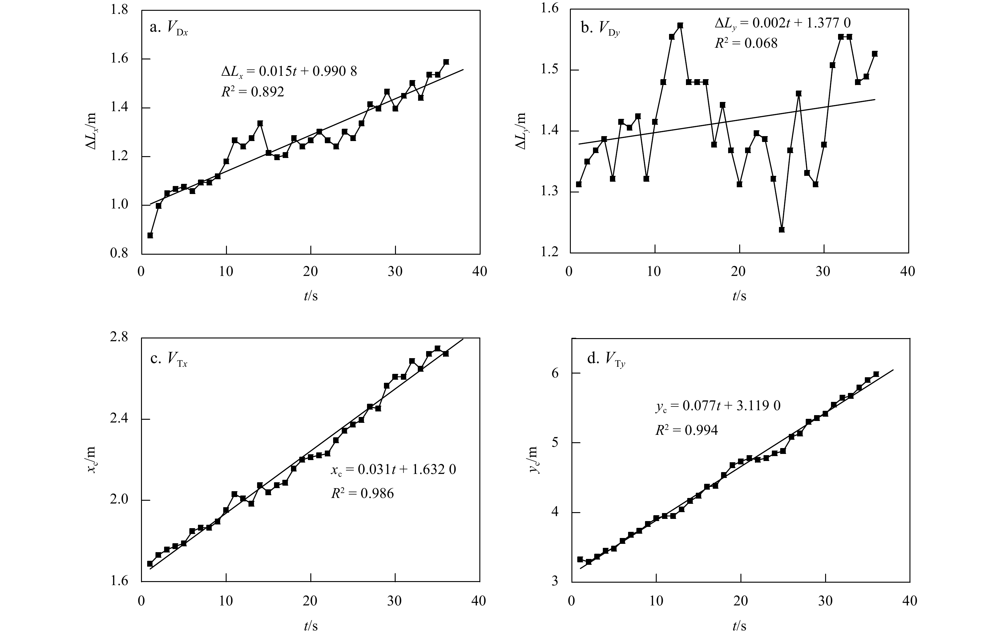
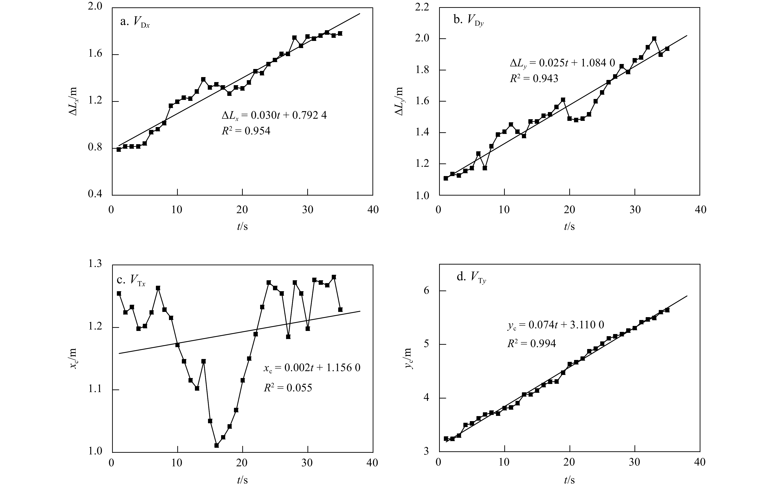
Figures 11–14 show the fitted results for Cases 1–4. In general, these correlation coefficients between the linear-fitted results and the measurement results are high. In addition to the


The estimated diffusion (
| Case | ${V_{ {\rm D}x} }/(\rm m \; \cdot \;\rm s^{ - 1})$ | ${V_{ {\rm D}y} }/(\rm m\; \cdot\; \rm s^{ - 1})$ | ${V_{ {\rm T}x} }/(\rm m \;\cdot \;\rm s^{ - 1})$ | ${V_{ {\rm T}y} }/(\rm m\; \cdot \;\rm s^{ - 1})$ | ${V_{\max} }/(\rm m \;\cdot\; \rm s^{ - 1})$ |
| 1 | 0.048 | 0.051 | 0.012 | 0.076 | 0.16 |
| 2 | 0.015 | * | 0.031 | 0.077 | 0.10 |
| 3 | 0.030 | 0.025 | * | 0.074 | 0.14 |
| 4 | 0.051 | 0.052 | 0.046 | 0.070 | 0.19 |
| Note: * denots a very low coefficient of determination (${R^2}$). | |||||
DownLoad:
CSV
We found that
The surf zone eddy shape patches occurred under Cases 1, 3, and 4, with an alongshore scale of approximately 2–4 m, 0.2–0.8 times the surf zone width; the cross-shore scale is roughly 1 m. The water depth was roughly 0.045 m at the dye release location. Therefore, the horizontal length scale was more significant than the water depth. These ratios of alongshore length scale to the surf zone width at the initial stage suggest that these present surf zone eddies are drastically different from those generated through the extrinsic mechanism of breaking wave vorticity forcing because they were formed at a smaller time scale. However, transient rips generated on alongshore uniform bathymetries are generally brief (2–5 min) and can migrate with an alongshore current (Castelle et al., 2016).
Moreover, according to the extrinsic mechanism, surf zone small-scale eddies due to wave breaking are hypothesized to coalesce and form larger eddies through nonlinear interactions, generating vortical motions in the surf zone over a wide range of spatial scales (Feddersen, 2014). Under similar incident wave conditions, numerical modeling demonstrated that vorticities of similar scales with the present occurred in the surf zone, and shear instability was crucial in generating these eddies. Section 4 presents the linear instability theory analysis performed to illustrate the horizontal length scales.
The analysis of the spatial scale of the surf zone eddy is hugely significant for validating the eddy generation mechanism. With the extrinsic mechanism, the small-scale eddies are hypothesized to coalesce and form larger eddies through nonlinear interactions, generating vortical motions in the surf zone over a wide range of spatial scales (from 10 m to 100 m) (Feddersen, 2014). However, according to linear instability theory, surf zone eddy can be generated more straight forwardly, agreeing with the present observation. There is a question about why the extrinsic mechanism can hardly explain the surf zone generation in a strong alongshore current. Further details are needed to explore in the future.
The 2D spatial scale of the surf zone eddy can be reflected straight with
Shear instability theory was first developed to explain the meandering motions observed in fields at 10–3–10–2 Hz frequencies and with wavelengths whose magnitude were too short to be gravity waves. Subsequently, shear instabilities of the mean alongshore current have been investigated based on a nonlinear shallow water equation with steady wave forcing (Allen et al., 1996; Noyes et al., 2005; Özkan-Haller and Kirby, 1999; Slinn et al., 1998). However, the effects of surf zone eddy induced by shear instability on dye transport patterns are poorly understood. Therefore, this section performs numerical analysis to validate whether the shear instability can induce perturbation velocity fields that may dominate the eddy patch deformation in the present strong alongshore current.
Shear instability theory has been described in detail elsewhere (Bowen and Holman, 1989; Dodd et al., 2004; Putrevu and Svendsen, 1992). Briefly, in a strong alongshore current, the uneven distribution of the time-average alongshore current
| $$ {\boldsymbol{u}}(x,y,t) = \big(u'{\text{(}}x,y,t{\text{),}}V{\text{(}}x{\text{) + }}v'{\text{(}}x,y,t)\big), $$ | (5) |
where
The shallow water, inviscid equations for horizontal momentum are as follows:
| $$ \nabla \cdot (h{\boldsymbol{u}}) = {\text{0}}, $$ | (6) |
| $$ {{\boldsymbol{u}}_t}{\text{ + (}}{\boldsymbol{u}} \cdot \nabla ){\boldsymbol{u}} + {{g}}\nabla \eta = {\text{0}} , $$ | (7) |
where
| $$ u' = - \frac{{{\psi _y}}}{h} = - \frac{{{\text{i}}\varphi k}}{h}{\text{exp(}}{\omega _{\text{i}}}t){\text{exp[i}}(ky - {\omega _{\text{r}}}t)] , $$ | (8) |
| $$ v' = \frac{{{\psi _x}}}{h} = \frac{{{\varphi _x}}}{h}{\text{exp(}}{\omega _{\text{i}}}t{\text{)exp[i}}(ky - {\omega _{\text{r}}}t)], $$ | (9) |
where
| $$ (V - c)\left({\varphi _{xx}} - {k^2}\varphi - \frac{{{\varphi _x}{h_x}}}{h}\right) - h\varphi {\left(\frac{{{V_x}}}{h}\right)_x} = {\text{0}} , $$ | (10) |
where
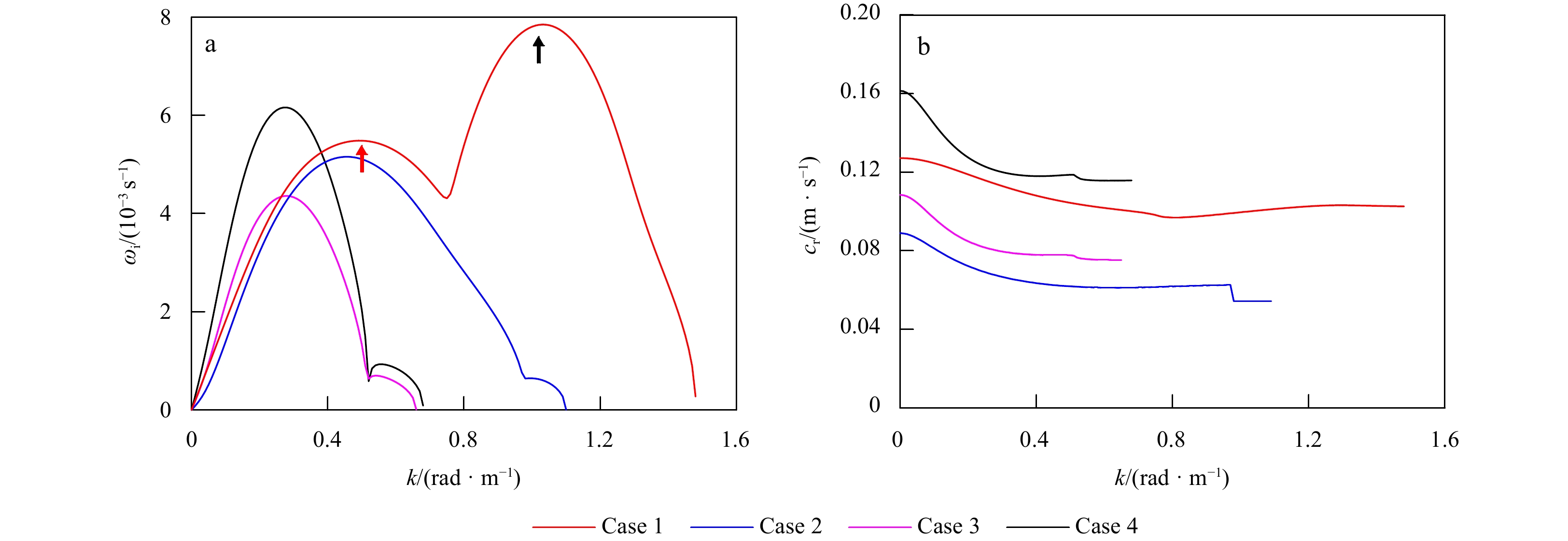
For a given water depth
The velocity profile of the mean longshore currents (fitted results) for Cases 1–4 (Fig. 6) was adopted as the background shear flows in the linear instability analysis, with the fitted lines in place of the discrete test data. Figure 16 shows the growth rate,

For Cases 1–4, the wave number (
| Case | ${k_{0,{\text{1} } } }$ | ${c_{ {\text{r,1} } } }$ | $ {T_{\text{1}}} $ | $ {L_1} $ | ${k_{0,{\text{2} } } }$ | ${c_{ {\text{r,2} } } }$ | $ {T_{\text{2}}} $ | $ {L_{\text{2}}} $ | |
| First mode | Second mode | ||||||||
| 1 | 0.490 | 0.105 | 122.41 | 12.82 | 1.030 | 0.100 | 60.93 | 6.10 | |
| 2 | 0.460 | 0.062 | 218.92 | 13.65 | 0.990 | 0.054 | 116.88 | 6.34 | |
| 3 | 0.280 | 0.080 | 279.48 | 22.43 | 0.620 | 0.076 | 133.28 | 10.13 | |
| 4 | 0.280 | 0.121 | 185.48 | 22.43 | 0.560 | 0.116 | 96.72 | 11.21 | |
DownLoad:
CSV
According to this analysis, the perturbation velocity field

The experimental measurement duration in this study was short, and the collecting range of dye patch movement was smaller than the field scale. Compared with the field test with long distance and long measurement time, other factors (such as wind, temperature, tide, etc.) (Kumar and Feddersen, 2017a, b) cannot be considered. On the other hand, image collecting and proceeding may bring errors in estimating the transport and diffusion due to experimental light and treatment technology of determining surf zone eddy patch boundary. In addition, while the results suggest the dominant plume behaviors are explained well by shear instability theory, aspects of the surf zone plume behavior may vary due to interaction with shelf processes, including Stokes drift, internal waves, fronts, and adjacent plumes.
The solid curves fitted to the results (Fig. 6) were used as input data for the linear instability analysis. However, the mean longshore current’s velocity profile significantly affected the instability mode (Ren et al., 2012). Also, different fitting methods may result in differences among these calculated perturbation velocity fields. They can be ignored due to the dominance of backshear to the shear instability mode. In other words, selected fitting methods have negligible effects on the backshear. Since the mean alongshore currents are regarded as being steady, only the calculated perturbation velocity fields are at the initial time given. However, nonlinear numerical modeling has demonstrated that the mixing induced by shear instability may adjust the velocity profile of the mean longshore current with time (Özkan-Haller and Kirby, 1999). Therefore, in the future, related numerical analysis should be conducted to investigate the time-dependent evolution of perturbation velocity induced by shear instability. In addition, numerical modeling with a phase-resolving Boussinesq-type wave model (such as funwaveC) (Feddersen et al., 2011) and a comparison between numerical and experimental results should be performed to diagnose the effect of shear instability with a strong current on dye patch transport in the surfzone. Such studies would allow for a more detailed understanding of the surf zone generation mechanism and address whether the surf zone eddy is dominated by shear instability rather than the breaking wave vorticity forcing or partly in a strong alongshore current.
In this paper, the evolution, propagation, and diffusion characteristics of surf zone eddies generated by shear instabilities were analyzed by dye patch tracing experiments. Also, the surf zone eddies generation mechanism was analyzed based on shear instability theory. The results demonstrated that under monochromatic unidirectional incident waves with a large angle of incidence, the surf zone eddies were generated in the shoreward and offshore directions on a plane beach. The eddy patches’ alongshore and cross-shore scale was approximately 4 m and 1 m, respectively.
We found that visible eddy or alongshore meandering patches occurred for the four test cases during the evolution of dye patches. These eddy patches were mainly transported in the alongshore direction. The alongshore propagation speed was approximately twice that of the cross-shore, and the cross-shore and alongshore diffusion speeds were weak (approximately 0.05 m/s). The development of these eddy patches can be roughly divided into two stages: in the initial stage, the eddy scale in both directions was about 0.1–0.2 times the width of the surf zone; in the stabilization stage, it was less than 0.2 times.
Based on shear instability theory, the perturbation velocity fields were obtained under the four wave conditions, showing that the velocity field structure was approximately consistent with the experimental observation. In addition, these velocity fields were more likely induced under random incident waves, which may drive double eddy. Consequently, the numerical analysis demonstrated that the linear instability theory could explain the transport evolution of observed eddy patches dominated by surf zone eddies in the strong alongshore current (Bowen and Holman, 1989; Brivois et al., 2012).
|
Abolfathi S, Cook S, Yeganeh-Bakhtiary A, et al. 2020. Microplastics transport and mixing mechanisms in the nearshore region. In: Lynett P J, ed. Proceedings of virtual Conference on Coastal Engineering, (36v): papers. 63, doi: 10.9753/icce.v36v.papers.63, https://icce-ojs-tamu.tdl.org/icce/article/view/10331 [2020-12-31/2023-05-01]
|
|
Abolfathi S, Pearson J. 2014. Solute dispersion in the nearshore due to oblique waves. In: Lynett P J, ed. Proceedings of 34th Conference on Coastal Engineering, (34): waves. 49, doi: 10.9753/icce.v34.waves.49, https://icce-ojs-tamu.tdl.org/icce/article/view/7803 [2014-10-30/2023-05-01]
|
|
Abolfathi S, Pearson J, 2017. Application of smoothed particle hydrodynamics (SPH) in nearshore mixing: a comparison to laboratory data. In: Lynett P J, ed. Proceedings of 35th Conference on Coastal Engineering, (35): currents. 16, doi: 10.9753/icce.v35.currents.16, https://icce-ojs-tamu.tdl.org/icce/article/view/8228 [2017-06-23/2023-05-01]
|
|
Allen J S, Newberger P A, Holman R A. 1996. Nonlinear shear instabilities of alongshore currents on plane beaches. Journal of Fluid Mechanics, 310: 181–213, doi: 10.1017/S002211209600 1772
|
|
Baquerizo A, Caballeria M, Losada M A, et al. 2001. Frontshear and backshear instabilities of the mean longshore current. Journal of Geophysical Research: Oceans, 106(C8): 16997–17011, doi: 10.1029/2001JC900004
|
|
Bowen A J, Holman R A. 1989. Shear instabilities of the mean longshore current: 1. Theory. Journal of Geophysical Research: Oceans, 94(C12): 18023–18030, doi: 10.1029/JC094iC12p18023
|
|
Brivois O, Idier D, Thiébot J, et al. 2012. On the use of linear stability model to characterize the morphological behaviour of a double bar system. Application to Truc Vert Beach (France). Comptes Rendus Geoscience, 344(5): 277–287, doi: 10.1016/j.crte.2012.02.004
|
|
Brown J A, MacMahan J H, Reniers A J H M, et al. 2015. Field observations of surf zone-inner shelf exchange on a rip-channeled beach. Journal of Physical Oceanography, 45(9): 2339–2355, doi: 10.1175/JPO-D-14-0118.1
|
|
Castelle B, Scott T, Brander R W, et al. 2016. Rip current types, circulation and hazard. Earth-Science Reviews, 163: 1–21, doi: 10.1016/j.earscirev.2016.09.008
|
|
Clark D B, Feddersen F, Guza R T. 2010. Cross-shore surfzone tracer dispersion in an alongshore current. Journal of Geophysical Research: Oceans, 115(C10): C10035, doi: 10.1029/2009JC005683
|
|
Clark D B, Feddersen F, Guza R T. 2011. Modeling surf zone tracer plumes: 2. Transport and dispersion. Journal of Geophysical Research: Oceans, 116(C11): C11028, doi: 10.1029/2011JC 007211
|
|
Clarke L B, Ackerman D, Largier J. 2007. Dye dispersion in the surf zone: measurements and simple models. Continental Shelf Research, 27(5): 650–669, doi: 10.1016/j.csr.2006.10.010
|
|
Dodd N, Iranzo V, Caballeria M. 2004. A subcritical instability of wave-driven alongshore currents. Journal of Geophysical Research: Oceans, 109(C2): C02018, doi: 10.1029/2001JC001106
|
|
Feddersen F. 1998. Weakly nonlinear shear waves. Journal of Fluid Mechanics, 372: 71–91, doi: 10.1017/S0022112098002158
|
|
Feddersen F. 2012. Scaling surf zone turbulence. Geophysical Research Letters, 39(18): L18613, doi: 10.1029/2012GL052970
|
|
Feddersen F. 2014. The generation of surfzone eddies in a strong alongshore current. Journal of Physical Oceanography, 44(2): 600–617, doi: 10.1175/JPO-D-13-051.1
|
|
Feddersen F, Clark D B, Guza R T. 2011. Modeling surf zone tracer plumes: 1. Waves, mean currents, and low-frequency eddies. Journal of Geophysical Research: Oceans, 116(C11): C11027, doi: 10.1029/2011JC007210
|
|
Grimes D J, Feddersen F, Giddings S N, et al. 2020a. Cross-shore deformation of a surfzone-released dye plume by an internal tide on the inner shelf. Journal of Physical Oceanography, 50(1): 35–54, doi: 10.1175/JPO-D-19-0046.1
|
|
Grimes D J, Feddersen F, Giddings S N. 2021. Long-distance/time surf-zone tracer evolution affected by inner-shelf tracer retention and recirculation. Journal of Geophysical Research: Oceans, 126(12): e2021JC017661, doi: 10.1029/2021JC017661
|
|
Grimes D J, Feddersen F, Kumar N. 2020b. Tracer exchange across the stratified inner-shelf driven by transient rip-currents and diurnal surface heat fluxes. Geophysical Research Letters, 47(10): e2019GL086501, doi: 10.1029/2019GL086501
|
|
Hally-Rosendahl K, Feddersen F. 2016. Modeling surfzone to inner-shelf tracer exchange. Journal of Geophysical Research: Oceans, 121(6): 4007–4025, doi: 10.1002/2015JC011530
|
|
Hally-Rosendahl K, Feddersen F, Clark D B, et al. 2015. Surfzone to inner-shelf exchange estimated from dye tracer balances. Journal of Geophysical Research: Oceans, 120(9): 6289–6308, doi: 10.1002/2015JC010844
|
|
Hally-Rosendahl K, Feddersen F, Guza R T. 2014. Cross-shore tracer exchange between the surfzone and inner-shelf. Journal of Geophysical Research: Oceans, 119(7): 4367–4388, doi: 10.1002/2013JC009722
|
|
Holland T K, Holman R A, Lippmann T C, et al. 1997. Practical use of video imagery in nearshore oceanographic field studies. IEEE Journal of Oceanic Engineering, 22(1): 81–92, doi: 10.1109/48.557542
|
|
Johnson D, Pattiaratchi C. 2004. Application, modelling and validation of surfzone drifters. Coastal Engineering, 51(5/6): 455–471, doi: 10.1016/j.coastaleng.2004.05.005
|
|
Kumar N, Feddersen F. 2017a. The effect of Stokes drift and transient rip currents on the inner shelf. Part I: no stratification. Journal of Physical Oceanography, 47(1): 227–241, doi: 10.1175/JPO-D-16-0076.1
|
|
Kumar N, Feddersen F. 2017b. The effect of stokes drift and transient rip currents on the inner shelf. Part II: with stratification. Journal of Physical Oceanography, 47(1): 243–260, doi: 10.1175/JPO-D-16-0077.1
|
|
Long J W, Özkan-Haller H T. 2009. Low-frequency characteristics of wave group–forced vortices. Journal of Geophysical Research: Oceans, 114(C8): C08004, doi: 10.1029/2008JC004894
|
|
Longuet-Higgins M S. 1970. Longshore currents generated by obliquely incident sea waves: 2. Journal of Geophysical Research, 75(33): 6790–6801, doi: 10.1029/JC075i033p06790
|
|
Moulton M, Chickadel C C, Thomson J. 2021. Warm and cool nearshore plumes connecting the surf zone to the inner shelf. Geophysical Research Letters, 48(10): e2020GL091675, doi: 10.1029/2020GL091675
|
|
Noyes T J, Guza R T, Elgar S, et al. 2004. Field observations of shear waves in the surf zone. Journal of Geophysical Research: Oceans, 109(C1): C01031, doi: 10.1029/2002JC001761
|
|
Noyes T J, Guza R T, Feddersen F, et al. 2005. Model-data comparisons of shear waves in the nearshore. Journal of Geophysical Research: Oceans, 110(C5): C05019, doi: 10.1029/2004JC002541
|
|
O’Dea A, Kumar N, Haller M C. 2021. Simulations of the surf zone eddy field and cross-shore exchange on a nonidealized bathymetry. Journal of Geophysical Research: Oceans, 126(5): e2020JC016619, doi: 10.1029/2020JC016619
|
|
Oltman-Shay J, Howd P A, Birkemeier W A. 1989. Shear instabilities of the mean longshore current: 2. field observations. Journal of Geophysical Research: Oceans, 94(C12): 18031–18042, doi: 10.1029/JC094iC12p18031
|
|
Özkan-Haller H T, Kirby J T. 1999. Nonlinear evolution of shear instabilities of the longshore current: a comparison of observations and computations. Journal of Geophysical Research: Oceans, 104(C11): 25953–25984, doi: 10.1029/1999JC900104
|
|
Pearson J M, Guymer I, West J R, et al. 2009. Solute mixing in the surf zone. Journal of Waterway, Port, Coastal, and Ocean Engineering, 135(4): 127–134, doi: 10.1061/(ASCE)0733-950X(2009)135:4(127
|
|
Peregrine D H. 1998. Surf zone currents. Theoretical and Computational Fluid Dynamics, 10(1–4): 295–309, doi: 10.1007/s001620050065
|
|
Putrevu U, Svendsen I A. 1992. Shear instability of longshore currents: a numerical study. Journal of Geophysical Research: Oceans, 97(C5): 7283–7303, doi: 10.1029/91JC02988
|
|
Ren Chunping, Zou Zhili, Qiu Dahong. 2012. Experimental study of the instabilities of alongshore currents on plane beaches. Coastal Engineering, 59(1): 72–89, doi: 10.1016/j.coastaleng.2011.07.004
|
|
Reniers A J H M, Battjes J A. 1997. A laboratory study of longshore currents over barred and non-barred beaches. Coastal Engineering, 30(1/2): 1–21, doi: 10.1016/S0378-3839(96)00033-6
|
|
Reniers A J H M, Battjes J A, Falqués A, et al. 1997. A laboratory study on the shear instability of longshore currents. Journal of Geophysical Research: Oceans, 102(C4): 8597–8609, doi: 10.1029/96JC03863
|
|
Reniers A J H M, Thornton E B, Stanton T P, et al. 2004. Vertical flow structure during Sandy Duck: observations and modeling. Coastal Engineering, 51(3): 237–260, doi: 10.1016/j.coastaleng.2004.02.001
|
|
Slinn D N, Allen J S, Newberger P A, et al. 1998. Nonlinear shear instabilities of alongshore currents over barred beaches. Journal of Geophysical Research: Oceans, 103(C9): 18357–18379, doi: 10.1029/98JC01111
|
|
Spydell M S. 2016. The suppression of surfzone cross-shore mixing by alongshore currents. Geophysical Research Letters, 43(18): 9781–9790, doi: 10.1002/2016GL070626
|
|
Spydell M S, Feddersen F. 2012a. A Lagrangian stochastic model of surf zone drifter dispersion. Journal of Geophysical Research: Oceans, 117(C3): C03041, doi: 10.1029/2011JC007701
|
|
Spydell M S, Feddersen F. 2012b. The effect of a non-zero Lagrangian time scale on bounded shear dispersion. Journal of Fluid Mechanics, 691: 69–94, doi: 10.1017/jfm.2011.443
|
|
Tang Jun, Lyu Yigang, Shen Yongming. 2016. Numerical simulation of the Kuroshio intrusion into the South China Sea by a passive tracer. Acta Oceanologica Sinica, 35(9): 111–116, doi: 10.1007/s13131-016-0932-8
|
|
Visser P J. 1991. Laboratory measurements of uniform longshore currents. Coastal Engineering, 15(5/6): 563–593, doi: 10.1016/0378-3839(91)90028-F
|
|
Wu Xiaodong, Feddersen F, Giddings S N, et al. 2020. Mechanisms of mid-to outer-shelf transport of shoreline-released tracers. Journal of Physical Oceanography, 50(7): 1813–1837, doi: 10.1175/JPO-D-19-0225.1
|
Figures(17) / Tables(4)

Supported by:
Beijing Renhe Information Technology Co. Ltd

Chunping Ren, Nannan Fu, Chong Yu, Yuchuan Bai, Kezhao Fang. Observing eddy dye patches induced by shear instabilities in the surf zone on a plane beach[J]. Acta Oceanologica Sinica, 2024, 43(3): 15-29. doi: 10.1007/s13131-023-2270-y

| VM | $x$/m | VM | $x$/m | |
| 1 | 2.0 | 9 | 6.0 | |
| 2 | 2.5 | 10 | 6.5 | |
| 3 | 3.0 | 11 | 7.0 | |
| 4 | 3.5 | 12 | 8.0 | |
| 5 | 4.0 | 13 | 9.0 | |
| 6 | 4.5 | 14 | 10.0 | |
| 7 | 5.0 | 15 | 11.0 | |
| 8 | 5.5 | 16 | 12.0 |
DownLoad:
CSV
| Case | Incident wave | Slope | D/cm | H/cm | T/s | xb/m | ${L_0}$ | ${\xi _{\text{0}}}$ | ${{{{H_0}} \mathord{\left/ {\vphantom {{{H_0}} L}} \right. } L}_0}$ |
| 1 | regular waves | 1:100 | 18 | 2.7 | 1.5 | 5.2 | 3.51 | 0.11 | 0.01 |
| 2 | irregular waves | 1:100 | 18 | 2.4 | 1.0 | 6.2 | 1.56 | 0.08 | 0.02 |
| 3 | irregular waves | 1:100 | 18 | 3.9 | 1.0 | 9.8 | 1.56 | 0.06 | 0.02 |
| 4 | irregular waves | 1:100 | 18 | 5.0 | 1.5 | 10.2 | 3.51 | 0.08 | 0.01 |
| Note: $D$, still water depth; $H$, mean wave height; $T$, peak period; ${L_0}$ and ${H_0}$, wave length and wave height at the wave maker, respectively; xb, surf-zone width. | |||||||||
DownLoad:
CSV
| Case | ${V_{ {\rm D}x} }/(\rm m \; \cdot \;\rm s^{ - 1})$ | ${V_{ {\rm D}y} }/(\rm m\; \cdot\; \rm s^{ - 1})$ | ${V_{ {\rm T}x} }/(\rm m \;\cdot \;\rm s^{ - 1})$ | ${V_{ {\rm T}y} }/(\rm m\; \cdot \;\rm s^{ - 1})$ | ${V_{\max} }/(\rm m \;\cdot\; \rm s^{ - 1})$ |
| 1 | 0.048 | 0.051 | 0.012 | 0.076 | 0.16 |
| 2 | 0.015 | * | 0.031 | 0.077 | 0.10 |
| 3 | 0.030 | 0.025 | * | 0.074 | 0.14 |
| 4 | 0.051 | 0.052 | 0.046 | 0.070 | 0.19 |
| Note: * denots a very low coefficient of determination (${R^2}$). | |||||
DownLoad:
CSV
| Case | ${k_{0,{\text{1} } } }$ | ${c_{ {\text{r,1} } } }$ | $ {T_{\text{1}}} $ | $ {L_1} $ | ${k_{0,{\text{2} } } }$ | ${c_{ {\text{r,2} } } }$ | $ {T_{\text{2}}} $ | $ {L_{\text{2}}} $ | |
| First mode | Second mode | ||||||||
| 1 | 0.490 | 0.105 | 122.41 | 12.82 | 1.030 | 0.100 | 60.93 | 6.10 | |
| 2 | 0.460 | 0.062 | 218.92 | 13.65 | 0.990 | 0.054 | 116.88 | 6.34 | |
| 3 | 0.280 | 0.080 | 279.48 | 22.43 | 0.620 | 0.076 | 133.28 | 10.13 | |
| 4 | 0.280 | 0.121 | 185.48 | 22.43 | 0.560 | 0.116 | 96.72 | 11.21 | |
DownLoad:
CSV
| VM | $x$/m | VM | $x$/m | |
| 1 | 2.0 | 9 | 6.0 | |
| 2 | 2.5 | 10 | 6.5 | |
| 3 | 3.0 | 11 | 7.0 | |
| 4 | 3.5 | 12 | 8.0 | |
| 5 | 4.0 | 13 | 9.0 | |
| 6 | 4.5 | 14 | 10.0 | |
| 7 | 5.0 | 15 | 11.0 | |
| 8 | 5.5 | 16 | 12.0 |
| Case | Incident wave | Slope | D/cm | H/cm | T/s | xb/m | ${L_0}$ | ${\xi _{\text{0}}}$ | ${{{{H_0}} \mathord{\left/ {\vphantom {{{H_0}} L}} \right. } L}_0}$ |
| 1 | regular waves | 1:100 | 18 | 2.7 | 1.5 | 5.2 | 3.51 | 0.11 | 0.01 |
| 2 | irregular waves | 1:100 | 18 | 2.4 | 1.0 | 6.2 | 1.56 | 0.08 | 0.02 |
| 3 | irregular waves | 1:100 | 18 | 3.9 | 1.0 | 9.8 | 1.56 | 0.06 | 0.02 |
| 4 | irregular waves | 1:100 | 18 | 5.0 | 1.5 | 10.2 | 3.51 | 0.08 | 0.01 |
| Note: $D$, still water depth; $H$, mean wave height; $T$, peak period; ${L_0}$ and ${H_0}$, wave length and wave height at the wave maker, respectively; xb, surf-zone width. | |||||||||
| Case | ${V_{ {\rm D}x} }/(\rm m \; \cdot \;\rm s^{ - 1})$ | ${V_{ {\rm D}y} }/(\rm m\; \cdot\; \rm s^{ - 1})$ | ${V_{ {\rm T}x} }/(\rm m \;\cdot \;\rm s^{ - 1})$ | ${V_{ {\rm T}y} }/(\rm m\; \cdot \;\rm s^{ - 1})$ | ${V_{\max} }/(\rm m \;\cdot\; \rm s^{ - 1})$ |
| 1 | 0.048 | 0.051 | 0.012 | 0.076 | 0.16 |
| 2 | 0.015 | * | 0.031 | 0.077 | 0.10 |
| 3 | 0.030 | 0.025 | * | 0.074 | 0.14 |
| 4 | 0.051 | 0.052 | 0.046 | 0.070 | 0.19 |
| Note: * denots a very low coefficient of determination (${R^2}$). | |||||
| Case | ${k_{0,{\text{1} } } }$ | ${c_{ {\text{r,1} } } }$ | $ {T_{\text{1}}} $ | $ {L_1} $ | ${k_{0,{\text{2} } } }$ | ${c_{ {\text{r,2} } } }$ | $ {T_{\text{2}}} $ | $ {L_{\text{2}}} $ | |
| First mode | Second mode | ||||||||
| 1 | 0.490 | 0.105 | 122.41 | 12.82 | 1.030 | 0.100 | 60.93 | 6.10 | |
| 2 | 0.460 | 0.062 | 218.92 | 13.65 | 0.990 | 0.054 | 116.88 | 6.34 | |
| 3 | 0.280 | 0.080 | 279.48 | 22.43 | 0.620 | 0.076 | 133.28 | 10.13 | |
| 4 | 0.280 | 0.121 | 185.48 | 22.43 | 0.560 | 0.116 | 96.72 | 11.21 | |
 DownLoad:


 DownLoad: