Study on the interannual variability of the Kerama Gap transport and its relation to the Kuroshio/Ryukyu Current system

1. Introduction

The Kuroshio Current originates from the northward branch of the North Equatorial Current at about 12°–15°N to the east of the Philippine coast. The majority of the Kuroshio enters the East China Sea (ECS) between Taiwan and Yonaguni-jima, the southernmost island of the Ryukyu Islands chain (RIC) (Andres et al., 2008). The current then exits the ECS through the Tokara Strait (Fig. 1). The Kuroshio current in the ECS, also known as the ECS-Kuroshio, is a surface-intensified, stable and continuous current. The remaining portion of the Kuroshio is blocked by the Ilan Ridge when it reaches Taiwan and diverts eastward, forming the subsurface-intensified Ryukyu Current, which has a flow core at depths ranging from 600 m to 900 m. The Ryukyu Current intensifies as it flows northeastward, being fed by the recirculation gyre and transports from the east (Nakamura et al., 2007; Thoppil et al., 2016; Zhao et al., 2020). Finally, the Ryukyu Current meets the ECS-Kuroshio as it exits the Tokara Strait. Unlike the ECS-Kuroshio, the Ryukyu Current is unstable and intermittent due to the influence of mesoscale eddies propagating from the Pacific Ocean (Jin et al., 2010; Zhu et al., 2010).

Figure  1.  Geographic location and bathymetry of the study area. Vectors represent the climatological mean (1950–2017) surface current field from the OGCM for the Earth Simulator (OFES). The shaded background color represents the water depth (unit: m, the water depth in the yellow area is very shallow). The black line indicates the location of the Kerama Gap. Two pink stars indicate the positions of the vertical potential density profiles on the both sides of the Kerama Gap, which are shown in Fig. 2. Ten red (blue) lines represent ten sections of the ECS-Kuroshio (Ryukyu) Current, while the cyan line denotes the location of the PN section.

DownLoad: Full-Size Img PowerPoint

The northeastward-flowing ECS-Kuroshio and Ryukyu Currents, mostly separated by the RIC, form a complete system, referred to as the Kuroshio/Ryukyu Current system. This system plays a crucial role in transporting heat, mass and nutrients from low to high latitudes, thereby shaping the climate and marine ecosystems along its path (Qiu and Chen, 2010; Guo et al., 2012; Wang and Wu, 2018; Gao et al., 2022). Therefore, gaining new insights into the Kuroshio/Ryukyu Current system can greatly benefit weather and climate prediction in the Pacific Ocean region.

The Kerama Gap is a narrow and deep waterway located between Okinawa Island and Miyako Island, with a depth that exceeds 1050 m and a width of 50 km. As the deepest channel in the RIC, the Kerama Gap transport (KGT) plays an important role in the mass and heat exchange between the ECS-Kuroshio and the Ryukyu Current (Nakamura et al., 2013; Nishina et al., 2016; Liu et al., 2020). Previous studies have highlighted the strong correlation between the KGT and the ECS-Kuroshio transport (Na et al., 2014; Soeyanto et al., 2014; Yu et al., 2015; Zhou et al., 2017). Furthermore, the temporal variability of the KGT has been reported to have a significant influence on the ECS Kuroshio (Na et al., 2014; Yu et al., 2015; Zhou et al., 2017). However, the relationship between the interannual variability of the KGT and the Kuroshio/Ryukyu Current system, especially between the KGT and the Ryukyu Current, requires further investigation. Given the limited duration of in-situ measurements (Yuan et al., 1998; Na et al., 2014), and the inability of remote sensing data to capture the subsurface-intensified Ryukyu Current and KGT, numerical modeling remains crucial in exploring this issue.

The high-frequency variability of the KGT, with an average period of about 120 days, is mainly caused by the difference in sea surface height (SSH) between the two sides of the Kerama Gap. Some studies have argued that the SSH difference is mainly caused by eddies on the ECS side, which are driven by the shift of the Kuroshio Current axis (Jin et al., 2010; Hsin et al., 2013; Zhou et al., 2018). Alternatively, other studies have proposed that mesoscale eddies from the northwestern Pacific can alter the SSH difference (Ichikawa et al., 2004; Soeyanto et al., 2014; Yu et al., 2015; Zhou et al., 2017). Yu et al. (2015) revealed that the seasonal cycle of the KGT is mainly driven by the local wind field. Regarding the multi-year variability, Zhou et al. (2018) proposed that the variability of the KGT is mainly determined by the SSH difference between the northeast and southwest of the Kerama Gap by using a 25-year ocean model, and the difference is dominated by the mesoscale eddies on the Pacific side. In addition, Yu et al. (2019) argued that the shift of the Kuroshio Current axis plays a secondary role in determining the SSH difference and the extreme flow of the KGT based on a 20-year reanalysis data. Liu et al. (2020) suggested that the multi-year variability of the KGT is dominated by a deep overflow, which correlates well with the density anomalies near its sill depth in the Philippine Sea, by analyzing three extreme deep overflow events with a 8-year ocean model data. In general, due to the limited data period, these studies of multi-year changes in KGT are all case studies of extreme flows. In addition, the dynamic mechanism is still under debate. Therefore, more research is needed to determine the changing law and dynamic mechanism of the interannual variability of the KGT and the Kuroshio/Ryukyu Current system.

This study addresses the following two questions: (1) What is the relationship between the KGT and the Kuroshio/Ryukyu Current system on an interannual time scale? (2) What is the physical mechanism controlling the interannual variability of the KGT and its associated currents? The rest of this paper is organized as follows. Section 2 describes the data used in this study and model validation. Section 3 introduces the employed methodologies. Key findings are presented in Section 4, and the conclusions and discussion are presented in Section 5.

2. Data and model validation

2.1 Numerical model output

The 68-year (from 1950 to 2017) monthly hindcast outputs of the OGCM for the Earth Simulator (OFES; Sasaki et al., 2004; Ram et al., 2022) are used in this study, including the potential temperature, salinity and horizontal velocity. The model has 54 vertical levels with varying layer thicknesses from 5 m near the surface to 330 m at a maximum depth of 6065 m, with a horizontal resolution of 0.1° in both longitude and latitude. The extensive time coverage is a significant advantage for studying interannual variability.

2.2 Observation data

Varieties of observations were used to validate the model results in the current study. The delayed-time level 4 gridded global sea level anomaly (SLA) data (1993–2017) are available from the Ssalto/Duacs multimission altimeter products, distributed by the Archiving, Validation, and Interpretation of Satellite Oceanographic (AVISO) data group and the Copernicus Marine Environment and Monitoring Service (CMEMS), with a horizontal resolution of about (1/3)° and a temporal resolution of daily. The objectively analyzed climatological mean (1955–2017) temperature and salinity data, based on the World Ocean Atlas 2018 (WOA 18), have a horizontal resolution of 0.25° × 0.25° and 102 levels from sea surface to 5500 m. The SLA obtained from tidal gauges can be accessed through the Permanent Service for Mean Sea Level (PSMSL).

2.3 Model validation

2.3.1   Mean state

The 68-year mean KGT determined by OFES is 0.6 × 10⁶ m³/s, with a larger standard deviation of 2.8 × 10⁶ m³/s. This indicates an alternate direction of the KGT, which is consistent with previous studies (Na et al., 2014; Zhou et al., 2018). Nevertheless, the average flow direction of the KGT points toward the Pacific Ocean, in contrast to earlier conclusions. According to Na et al. (2014), the average KGT is approximately 2.0 × 10⁶ m³/s, with a westward flow towards the ECS, based on a 2-year observational dataset including Current and Pressure-Recording Inverted Echo Sounders (CPIES) and moored current meters. The intrusion of the mean flow into the ECS via the Kerema Gap is believed to comprise of two components. One is the intrusion of low-salinity North Pacific Intermediate Water (NPIW) (Nakamura et al., 2013). Zhou et al. (2018) identified the subsurface-intensified flow core around 500 m using the observations of Na et al. (2014) and a Hybrid Coordinate Ocean Model (HYCOM) product. The other part is a bottom-enhanced overflow, which is thought sustained by the deep density difference between the two sides of the Kerama Gap (Nakamura et al., 2013).

To examine the difference between the model-inferred mean flows and observations, a vertical section of mean velocity through the Kerama Gap is presented (Fig. 2a). In the model, the topography of Kerama Gap consists of a wide and shallow portion and a narrow and deep portion, with a maximum depth of 900 m. Both the WOA 18-based observations and the model reveal the presence of a deep density bifurcation, which is believed to be responsible for sustaining the deep overflow, occurring at depths exceeding 900 m (Figs 2b and c). It can be inferred that the OFES does not account for the deep overflow as it underestimates the actual depth of the Kerama Gap. This will undoubtedly affect the modelling of the mean flow. Nonetheless, we believe that the lack of this overflow should not be the primary reason for the model’s underestimation of the mean flow into the ECS. This is due to the fact that neither the observations nor the model indicate that this overflow exceeds 0.4 × 10⁶ m³/s (Nishina et al., 2016; Liu et al., 2020), which is much smaller than the average observational KGT (2.0 × 10⁶ m³/s). In addition, the absence of overflow also has no effect on our investigations of interannual variability since the deep density bifurcation is highly stable.

Figure  2.  Vertical section of the long-term mean velocity (unit: m/s) through the Kerama Gap derived from OFES (a), and a comparison of two long-term mean (1955–2017) vertical potential density profiles on both sides of the Kerama Gap derived from WOA 18 (b) and derived from OFES (c). In a, positive values indicate the flow towards the Pacific Ocean, and distance was measured from the southwestern end of the section depicted in Fig. 1. For b and c, the locations are shown in Fig. 1 (two pink stars), and the red (blue) lines represent the profiles on the Pacific (ECS) side.

DownLoad: Full-Size Img PowerPoint

We speculate that the systematic error of the mean flow is mainly come from the underestimation of the intermediate water intrusion. It is clear that in Fig. 2a there is a subsurface core between 400 m and 700 m, which is directed towards the Pacific side. The position of this flow core is consistent with previous conclusions (Na et al., 2014; Zhou et al., 2018), but in the opposite direction. The principal cause of this systematic error remains unknown. It could be associated with the intrinsic dynamics of the OFES model. However, we persist that this will not impact our examination of the interannual variability of the Kuroshio/Ryukyu Current system and its dynamic mechanisms for the following two reasons. Firstly, Section 2.3.2 confirmed that the model is capable of representing the transport fluctuations within the Kuroshio/Ryukyu Current system. Secondly, Section 5 presents evidence that the laws and dynamical mechanisms discovered in this work are robust through using remotely sensed SLA data.

2.3.2   Variability

To verify the accuracy of the model in replicating the temporal variability within the Kuroshio/Ryukyu Current system, we initially compared the modelled KGT with the 2-year observations from Na et al. (2014) and the Ryukyu Current transport with the 2-year observations from Zhao et al. (2020). These observations were interpolated into monthly results through cubic spline interpolation for comparison with the OFES.

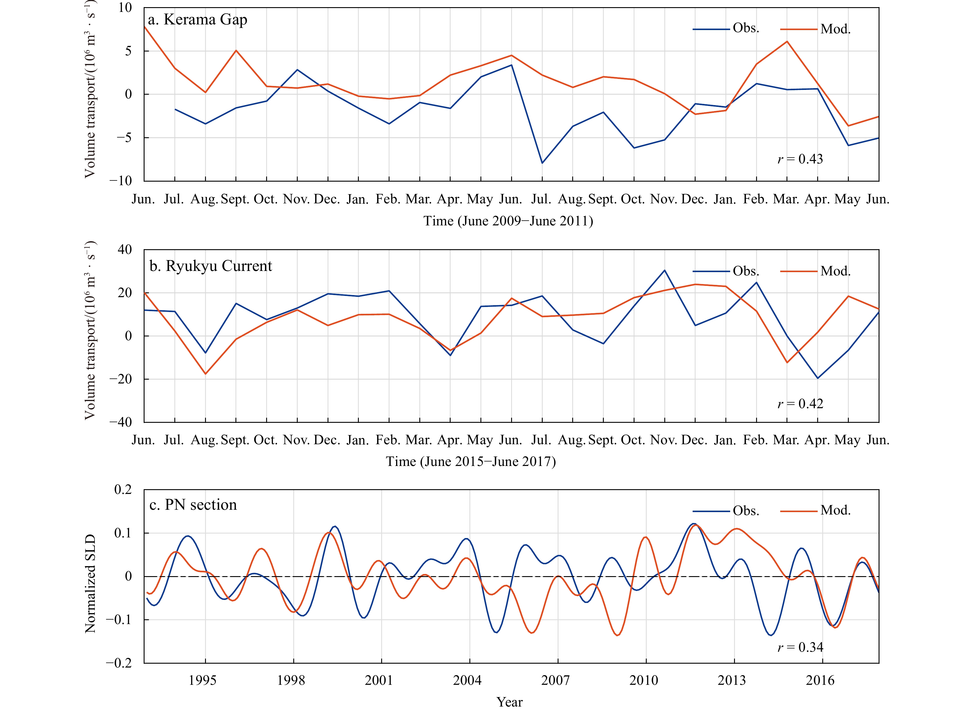
Figure 3a shows a bias between the observations and model for the KGT, which is consistent with previous findings in the mean flow. The model indicated a mean of 1.2 × 10⁶ m³/s, while the observations showed a mean transport of –1.7 × 10⁶ m³/s. It is worth noting that, in this study, the KGT towards the Pacific side is set to be positive. Although there is a systematic bias in the mean transport, their correlation coefficient is 0.43, which is significant at 90% confidence level, meanwhile the standard deviation of the model’s KGT is 2.7 × 10⁶ m³/s, which is comparable to the observed results (2.9 × 10⁶ m³/s). For the Ryukyu Current (Fig. 3b), the model predicts a transport of (8.4 ± 10.6) × 10⁶ m³/s, which concurs with the observational result ((9.0 ± 11.6) × 10⁶ m³/s). Furthermore, the correlation between the model and observations is also statistically significant.

Figure  3.  Comparison of the transport between the observations (Obs., blue) and the model (Mod., red) (a and b) and normalized sea level difference (SLD) for the PN section (c) . a. Two-year KGT from June 2009 to June 2011, and the observational time series is from Na et al. (2014). b. Two-year Ryukyu Current transport from June 2015 to June 2017, and the observational time series is from Zhao et al. (2020).

DownLoad: Full-Size Img PowerPoint

Long-term monitoring of the Kuroshio/Ryukyu Current system is significantly restricted. In order to evaluate the model’s ability to simulate the interannual variability, the remotely sensed SLA data can be used to validate the surface geostrophic current. As only the ECS-Kuroshio is surface-intenfised, the PN section, shown in Fig. 1, is picked for comparison. Figure 3c shows the interannual variability of the normalized sea level difference (SLD) between the individual endpoints of the PN section (in this study, the interannual variability is extracted from the raw time series using a 13-month low-pass filter). The interannual variability of the SLD derived from OFES is in good agreement with the observations, with a correlation coefficient of 0.34 (significant at 90% significance level). To extend the validation period, we have selected two gauge stations on the Ryukyu Island chain: Naha (26.21°N, 127.67°E) and Nisinoomote (30.74°N, 131.00°E). They will be used to test the model’s ability to capture the interannual variability of the SLA. The data covers the period from July 1966 to December 2017 in Naha, and from April 1965 to December 2017 in Nisinoomote. The correlation coefficients between the observation and model are 0.28 for Naha and 0.27 for Nisinoomote, respectively. Both are statistically significant at a 95% confidence level (figure not shown).

We thus conclude that the systematic bias is limited to the representation of the mean flow of the KGT and has no effect on the model’s ability to accurately represent the variability of the Kuroshio/Ryukyu Current system.

3. Methodology

Song (2006) developed a simple method to estimate the interbasin transport through a narrow strait for an ideal two-layer fluid. It has been successfully used to estimate the interbasin exchange of water masses in Asian marginal seas, such as the Makassar Strait, Luzon Strait, and the Korea/Tsushima Strait (Song, 2006). This estimation is achieved by combining the “geostrophic control” formula of Garrett and Toulany (1982) and the “hydraulic control” theory introduced by Whitehead et al. (1974):

It has been successfully used to estimate the interbasin exchange of water masses in Asian marginal seas, such as the Makassar Strait, Luzon Strait and the Tsushima Strait (Song, 2006).

In Eq. (1), $ {Q}_{\mathrm{g}} $ represents the volume flux in the upper layer, which is mainly influenced by the SSH difference, $\Delta \eta ={\eta }_{\mathrm{u}}-{\eta }_{\mathrm{d}} $, between two connected water bodies:

where $ f $ is the Coriolis parameter; $ g $ is the gravitational acceleration, $ {\eta }_{\mathrm{u}} $ and $ {\eta }_{\mathrm{d}} $ are the upstream and downstream SSH, respectively; and $ {H}_{1} $ is the upper layer thickness. The theoretical justification of the formulation has been discussed by Garrett and Toulany (1982).

$ {Q}_{\mathrm{h}} $ stands for the transport of the lower layer through the strait. If the width of the passage (L) is greater than the local baroclinic Rossby radius of deformation, $ R={\left(\dfrac{2{g}' \mathrm{\Delta }h}{{f}^{2}}\right)}^{1/2} $, $ {Q}_{\mathrm{h}} $ can be predicted by

where $ {H}_{2} $ is the thickness of the lower layer, $ {g}'=\dfrac{g\mathrm{\Delta }\rho }{\rho } $ is the reduced gravity, $ \rho $ and $\rho + \Delta \rho $ are the densities in the upper and lower layers, and $ \Delta h={h}_{\mathrm{u}}-{h}_{\mathrm{d}} $ is the difference between the upstream and downstream interface heights above the sill tip. Otherwise, when $ L < R $, the $ {Q}_{\mathrm{h}} $ is calculated by

It should be emphasized that the expressions of $ {Q}_{\mathrm{h}} $ are derived from the hydraulic control theory of Whitehead et al. (1974). They have been found to be effective in explaining the bottom-intensified deep overflow through a strait (Qu et al., 2006; Qu and Song, 2009; Susanto and Song, 2015; Liu et al., 2020). In this theory, the upper layer is stationary, and the lower layer transport is mainly driven by the pressure head between the two connected water bodies, which is dominated by $ \Delta h $. In fact, the expressions of Whitehead et al. (1974) can be re-established by setting $ \Delta \eta =0 $ and $ {H}_{2}=\Delta h $ in the above equation.

4. Results

4.1 Interannual variability of the KGT and its relation to the Kuroshio/Ryukyu Current system

To represent the transport structure of the ECS-Kuroshio and the Ryukyu Current, ten sections have been selected from each of these two currents (red and blue lines in Fig. 1). The sections crossing the ECS-Kuroshio are positioned perpendicular to the main axis of the ECS-Kuroshio, which is determined by tracking the local maximum speed of the climatological mean surface velocity obtained from OFES. The end points of the section are defined as the position where the velocity magnitude is 10% of the main axis velocity. The Kuroshio is relatively stable and is essentially confined in the Okinawa Trough, which can be covered by our defined sections. On the other hand, the Ryukyu Current exhibits high instability. To encompass the current axis shift, the sections crossing the Ryukyu Current are positioned perpendicular to the RIC, and extended from the RIC to the continental slope at a depth of 2500 m.

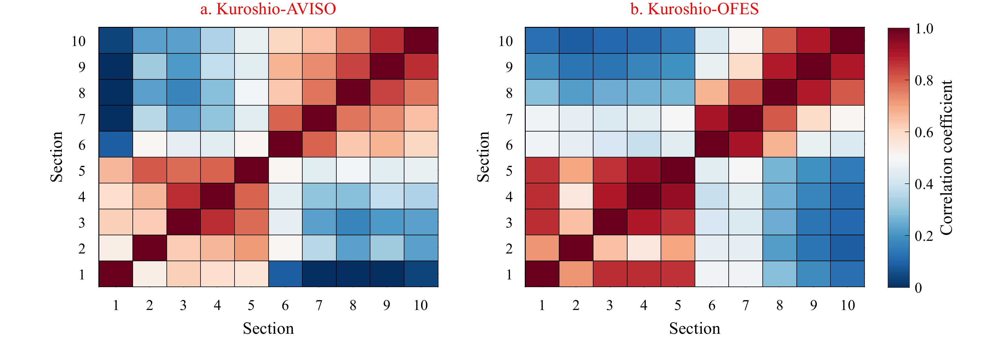
Figure 4a displays the correlogram of the interannual variability of the surface geostrophic transport through the ten ECS-Kuroshio sections, which is derived from altimeter data. The surface geostrophic transport refers to the integration of the surface geostrophic velocity over the section. The correlogram shows that there are high correlations exist between the first five or last five sections, with an average correlation coefficient greater than 0.50, at the 99% significance level. On the other hand, the correlations between the first five sections and the last five sections decrease significantly, with an average correlation coefficient of 0.31. These results suggest that there is a clear shift in the correlation between Sections 5 and 6. Similarly, Fig. 4b shows the OFES results, which also reveal a clear shift in the correlation between Sections 5 and 6. It is important to note that the Ryukyu Current is enhanced in the subsurface layer, and thus no similar structure was detected from the surface geostrophic transport of the Ryukyu Current.

Figure  4.  Correlogram of the interannual variability of the surface geostrophic transport for the ten Kuroshio sections estimated from AVISO data (a) and OFES output (b) during 1993 to 2017, respectively.

DownLoad: Full-Size Img PowerPoint

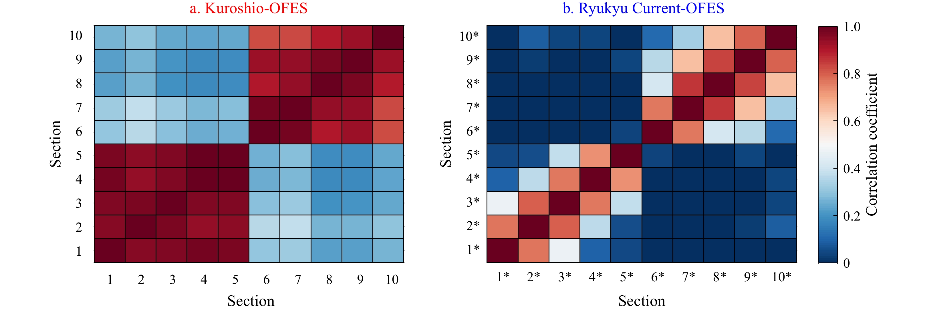
The vertically integrated volume transports of the ECS-Kuroshio and the Ryukyu Current are calculated using the 3-dimensional velocity field output from OFES. Compared with the surface geostrophic transports shown in Fig. 4b, the correlation coefficients for the vertically integrated results increase significantly between any two sections for the ECS-Kuroshio (Fig. 5a). However, there is still a noticeable difference between the upstream and downstream sections, as the average correlation coefficient drops from about 0.97 between the first five or last five sections to about 0.39 between the first five and last five sections. It is worth noting that the interannual time series of the transport through five upstream or downstream sections almost overlap (figure not shown), indicating that the upstream and downstream of the ECS-Kuroshio are relatively stable, and the water exchange with the ECS has little influence on the interannual variability of the ECS-Kuroshio.

Figure  5.  Correlogram of the interannual variability of the vertical integrated volume transport for the ten sections of Kuroshio (a) and Ryukyu Current (b) estimated from the OFES outputs during 1993 to 2017, respectively.

DownLoad: Full-Size Img PowerPoint

Despite the fact that the transport of the Ryukyu Current is known to be quite unstable and heavily influenced by the recirculation gyre and transport from the east, it is surprising to find that similar structures can also be found in the Ryukyu Current (Fig. 5b). The correlation coefficients between the first five or last five sections are mostly significant at the 99% confidence level, with a mean value of approximately 0.52. In contrast, none of the correlation coefficients between the first five and the last five sections are significant at the 95% confidence level, and most of them even show weak negative correlations, with a mean value of approximately –0.06. Considering that the Kerama Gap is located exactly between Sections 5 and 6 (Fig. 1), it is easy to speculate that the interannual variability of the KGT should be related to the interannual variability of the upstream and downstream transport of the Kuroshio/Ryukyu Current system.

To better understand the relationship between the interannual variability of the KGT and the Kuroshio/Ryukyu Current system, we obtained the interannual time series of the KGT (Fig. 6a) and calculated the correlation coefficients with the transports through the ten sections of the ECS-Kuroshio and Ryukyu Current (Table 1). It should be noted that the subsequent discussion regarding interannual variability exclusively pertains to the 68-year monthly output from OFES. Therefore, here we provide a consistent standard for testing the statistical significance of correlation coefficients. Using a Student’s t-test and accounting for the sample size, we find that the t-value is 0.27 at the 95% significance level and 0.35 at the 99% significance level. The KGT is strongly positively correlated with the upstream sections of the ECS-Kuroshio, with correlation coefficients that are significant at the 99% confidence level (Table 1). However, it has a weak negative correlation with the downstream ECS-Kuroshio, with all correlation coefficients being less than 99% confident. The characteristics of the Ryukyu Current are similar to those of the Kuroshio, with positive correlations for the upstream and negative correlations for the downstream. Almost all the correlation coefficients for the Ryukyu Current are significant at the 99% confidence level.

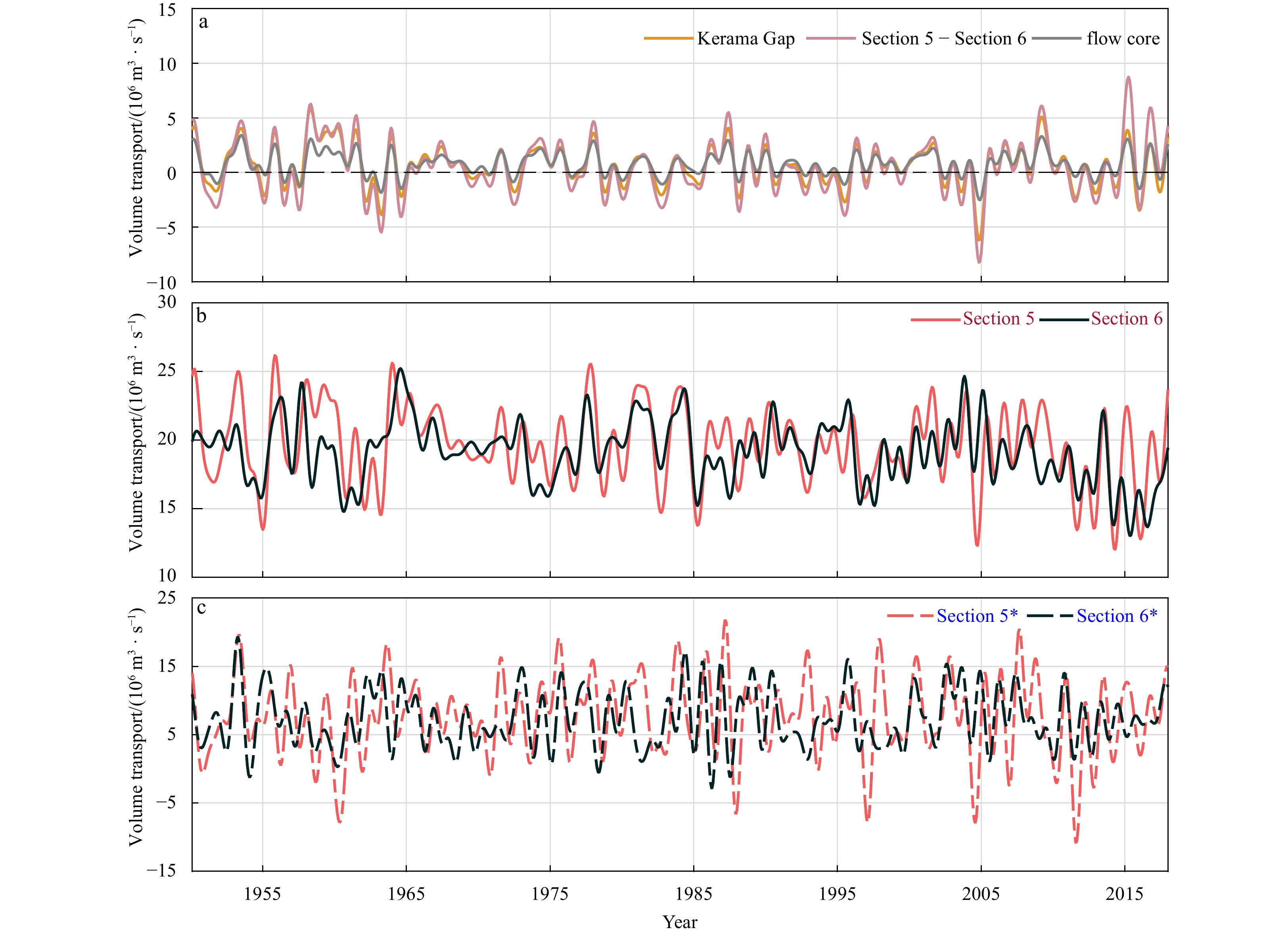
Figure  6.  The interannual variability of the volume transport through the Kerama Gap (eastward is positive) and the difference between the Section 5 and Section 6 of the ECS-Kuroshio (red) (a), the interannual variability of the volume transport through Section 5 (upstream) and Section 6 (downstream) of the ECS-Kuroshio (northward is positive) (b), and the interannual variability of the volume transport through Section 5* (upstream) and Section 6* (downstream) of the Ryukyu Current (northward is positive) (c) during 1950–2017. In a, the gray line represents the volume transport of the deep flow core between 400 m and 700 m.

DownLoad: Full-Size Img PowerPoint

Table  1.  Correlation coefficients between the KGT and ten sections of the vertically integrated volume transport for ECS-Kuroshio and Ryukyu Current

Section	Correlation coefficient
	ECS-Kuroshio	Ryukyu Current
1	0.68	0.46
2	0.62	0.43
3	0.70	0.50
4	0.74	0.48
5	0.74	0.33
6	–0.27	–0.27
7	–0.25	–0.49
8	–0.30	–0.53
9	–0.31	–0.37
10	–0.33	–0.42
Note: The bold correlation coefficient values are significant at the 99% significance level.

 | Show Table

DownLoad: CSV

A composite analysis was performed by subtracting the mean vertical integrated volume transport for the negative KGT period from the positive KGT period (Fig. 7). The results of the composite analysis show the same relationship between the KGT and the Kuroshio/Ryukyu Current system as described in Table 1. That is, the positive phase of the KGT is typically associated with an increase in the upstream ECS-Kuroshio and Ryukyu Current and a decrease in the downstream Ryukyu Current. Additionally, an offshore current running parallel to the latitude of the Kerama Gap is found, which is accompanied by a prominent anticyclonic vortex located to the south of the Kerama Gap.

Figure  7.  Composite analysis of the vertical integrated volume transport (unit: 10⁶ m³/s) for the Kuroshio/Ryukyu Current system using the difference between the positive and negative phase of the KGT (Fig. 6a). Red vectors represent the local transport exceeding the 99% significant level. The two 1° × 1° boxes indicate the region for the calculation of the $ \Delta \eta $ and $ \Delta h $. The centers of the ECS and Pacific regions are 26.7°N, 126.4°E and 24.1°N, 127.1°E, respectively.

DownLoad: Full-Size Img PowerPoint

To quantify the contribution of the KGT to the Kuroshio/Ryukyu Current system, Figs 6b and c present the interannual variability of the volume transport through Sections 5 and 6 for the ECS-Kuroshio and the Ryukyu Current, respectively. The ECS-Kuroshio section shows a continuous northward flow, with a mean transport of 17.1 × 10⁶ m³/s and a standard deviation of 2.2 × 10⁶ m³/s (Fig. 6b). This finding is consistent with previous observations reported by Andres et al. (2008). On the other hand, the Ryukyu Current has a mean transport of 7.9 × 10⁶ m³/s (Fig. 6c), which is relatively smaller than that of the ECS-Kuroshio. However, the standard deviation of the Ryukyu Current is as high as 10.4 × 10⁶ m³/s, indicating its inherent instability, which can sometimes cause it to flow in the opposite direction. This result is also consistent with previous observations (Zhu et al., 2003).

The transport difference between Sections 5 and 6 for the ECS-Kuroshio is almost identical to the interannual variability of the KGT (Fig. 6a), with a high correlation coefficient of 0.97. It suggests that the interannual variability of the difference between the upstream and downstream regions of the ECS-Kuroshio is entirely due to the variability of the KGT. Moreover, the interannual variability of the KGT contributes significantly to the variability of the ECS-Kuroshio itself, as the standard deviation of the KGT (2.8 × 10⁶ m³/s) is comparable to that of the ECS-Kuroshio (2.2 × 10⁶ m³/s). On the other hand, although there is an obvious relationship between the interannual variability of the Ryukyu Current and the KGT (Table 1 and Fig. 7), the contribution of the KGT to the interannual variability of the Ryukyu Current is thought to be limited. This is because the standard deviation of the KGT (2.8 × 10⁶ m³/s) is about 37% of the standard deviation of the average Ryukyu Current transport through Sections 5* and 6* (6.9 × 10⁶ m³/s) and the difference between Sections 5* and 6* of the Ryukyu Current (8.1 × 10⁶ m³/s). The interannual variation of the Ryukyu Current is mostly due to the variation in the offshore currents induced by the anticyclonic vortex shown in Fig. 7. The dynamic mechanism of the interannual variability of the KGT and the associated Kuroshio/Ryukyu Current system is discussed in the next section.

4.2 Dynamic mechanism for the interannual variability

As shown in Fig. 2a, the velocity of water flow through the Kerama Gap exhibits a subsurface-intensified structure. The subsurface flow core is located between 400 m and 700 m. In Fig. 6a, the transport of the flow core, which is obtained by integrating the velocity between 400 m and 700 m, is strongly correlated with the total transport, accounting for almost 85% of the standard deviation. This suggests that the interannual variability of the KGT is mainly dominated by the variability of the subsurface-intensified flow core.

To further quantify the dynamic processes, we calculated the interannual variability of the KGT using Eq. (1). The width of the Kerama Gap is approximately 50 km, which is comparable to the local baroclinic Rossby radius of deformation (Chelton et al., 1998). Therefore, Q_h is calculated using Eq. (3). For this calculation, the interface is chosen as the 25.5 kg/m³ isopycnal, which is essentially the base of the pycnocline. The 25.5 kg/m³ isopycnal lies at a depth of about 400 m. Hence, the value of H₁ is set at 400 m. Since the total depth of the sill is 900 m, so H₂ is defined as 500 m. The two regions for the calculation of $ \Delta \eta $ and $ \Delta h $ are shown in Fig. 7. In this study, the KGT from the ECS to the Pacific Ocean is defined as positive. Therefore, $ {\eta }_{\mathrm{u}} $ and $ {h}_{\mathrm{u}} $ represent the values for the ECS side, while $ {\eta }_{\mathrm{d}} $ and h_d represent the values for the Pacific side.

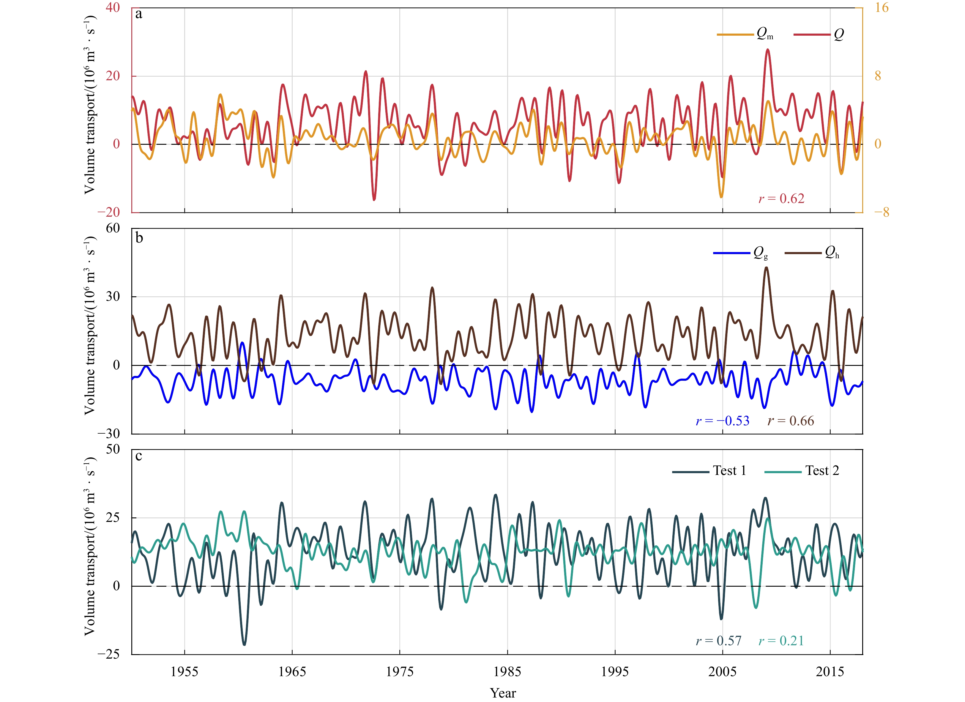
Figure 8a compares the interannual variability of the KGT between the results derived from the OFES velocity field, Q_m, and the theory, Q. The standard deviation of Q is 6.6 × 10⁶ m³/s, which is about twice that of Q_m (2.8 × 10⁶ m³/s). The discrepancy is largely due to the friction associated with the complex topography in the Kerama Gap. Q shows a strong correlation with Q_m, with a significant correlation coefficient of 0.62 at the 99% level, which proves that the interannual variation of the KGT can be well explained by this theory.

Figure  8.  Comparison of the interannual variability of Q_m (orange) and Q (red) (a), comparison of the interannual variability of Q_g (blue) and Q_h (brown) (b), and two sensitivity test results including holding h_u constant (Test 1; dark green) and holding h_d constant (Test 2; light green) (c). For a, the correlation coefficient is shown at the bottom; for b and c, the correlation coefficients between the two series and Q_m and between the two tests and Q_m are shown at the bottom, respectively.

DownLoad: Full-Size Img PowerPoint

Figure 8b shows that Q_h is positively correlated with Q and Q_m, and the correlation coefficient between Q_h and Q_m can reach 0.66. The standard deviation of Q_h is 8.7 × 10⁶ m³/s, which is slightly larger than that of Q (6.6 × 10⁶ m³/s). On the other hand, Q_g shows a negative correlation with Q and Q_m, with a correlation coefficient between Q_g and Q_m of –0.53. The standard deviation of Q_g is 4.5 × 10⁶ m³/s, which is only half of that of Q. These results show that the interannual variability of KGT is mainly controlled by the interface height difference, $ \Delta h $, and not by the SSH difference, $ \Delta \eta $. In addition, it can be speculated that $ \Delta \eta $ would induce a weaker upper layer flow in the opposite direction to the KGT.

Two sensitivity experiments were also carried out to assess the contributions of h_u and h_d to the KGT. As shown in Fig. 8c, Test 1, where h_u is held constant, shows a higher correlation coefficient of 0.57, which is significant at the 99% level. In contrast, Test 2 held h_d constant. The correlation coefficient for Test 2 is much lower (0.21), below the 95% level of significance. This indicates that interface height variations on the Pacific side play a more crucial role in controlling the interannual variability of the KGT than those on the ECS side.

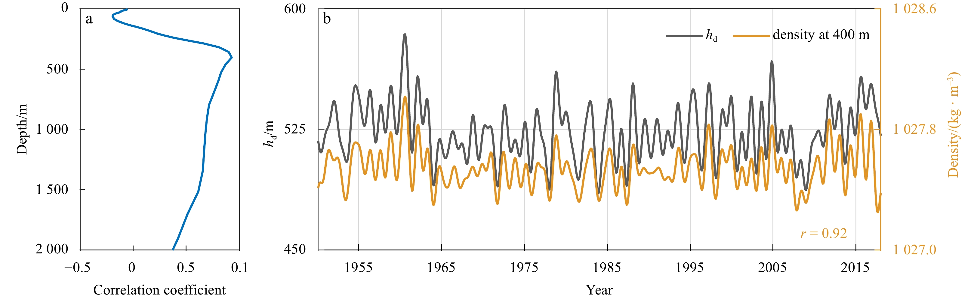
According to Whitehead et al. (1974), the variation of h is mainly dominated by the subsurface density anomalies, which can be confirmed by Fig. 9. Figure 9a illustrates the correlation coefficient between h_d and the local density anomalies at different depths. The maximum correlation coefficient is as high as 0.92, which is exactly located at about 400 m. On the contrary, there is a weak negative correlation between h_d and the surface density anomalies. As shown in Fig. 9b, h_d, which is believed to control the interannual variability of the KGT, shows exactly the same interannual variation as the local density anomalies at 400 m.

Figure  9.  Correlation coefficient between $ {h}_{\mathrm{d}} $ and the local density anomalies at different depths (a), and comparison of the interannual variability of $ {h}_{\mathrm{d}} $ (gray) and local density anomalies at 400 m (yellow) (b). The correlation coefficient is shown at the bottom in b.

DownLoad: Full-Size Img PowerPoint

To further identify the source of the subsurface density anomaly signals located to the south of the Kerama Gap, Fig. 10 shows the time-longitude variability of the subsurface density anomalies along the latitude of 24.1°N (shown in Fig. 11a) from 1950 to 2017. The majority of the anomaly signals are found to propagate from the east. Based on the slope of the signal propagation in Fig. 10, the propagation speed of the subsurface density anomaly signals can be estimated to be about 7.4 km/d, which is consistent with the speed of the local first-order baroclinic Rossby wave. Thus, these westward propagating signals are likely generated by Rossby waves or mesoscale eddies, which are not well separated in this study and are not the focus of this paper. It has been confirmed that these signals are not associated with the subsurface mode water, which usually moves in a southwesterly direction and at a slower speed compared to the Rossby waves (Xu et al., 2014, 2016).

Figure  10.  Time-dependent density anomaly at 400 m during 1950–2017 along the path shown in Fig. 11a.

DownLoad: Full-Size Img PowerPoint

Figure  11.  Composite analysis of the density anomaly (shaded; unit: kg/m³) and horizontal velocity (vector; unit: m/s) at a depth of 400 m, with time leads 8 months (a), 6 months (b), 4 months (c), 2 months (d), and 0 month (e) for the positive KGT year, and the density anomaly and horizontal velocity at a depth of 400 m, with time leads 8 months (f), 6 months (g), 4 months (h), 2 months (i), and 0 month (j) for the negative KGT year. Only the negative density anomaly signals are shown in a–e and only the positive density anomaly signals are shown in f–j. The green line with stars in Fig. 11a represents the path followed to track the westward propagating density anomaly signals. The black line in Fig. 11b shows the section used to plot the vertical distribution of the density anomaly signals (Fig. 12). Ten yellow (purple) lines represent the propagation location of negative (positive) density anomaly signals.

DownLoad: Full-Size Img PowerPoint

Figure 11 depicts the results of a composite analysis with time leads ranging from 8 months to 0 month, for both the positive and negative phases of the KGT. Taking the positive KGT as an example, negative density anomaly signals are evident at about 137°E, preceding the strongest positive KGT by 8 months (Fig. 11a). These signals gradually propagate westwards along the latitude band from 22°N to 26°N, with the leading signals first reaching the region south of the Kerama Gap about 4 months later (Fig. 11c). Subsequently, the other signals arrive and increase the density anomaly. Notably, the negative density anomaly signals can enter the ECS and eventually occupy the spatial region from 22°N to 26°N and 123°E to 132°E (Fig. 11e), which corresponds to the region of the anticyclonic vortex shown in Fig. 7. When these negative density anomaly signals reach their maximum, the accompanying anticyclonic vortex also reaches its maximum strength over the same region. As a result, the upstream ECS-Kuroshio, the upstream Ryukyu Current and the KGT all intensify. In addition, the anticyclonic vortex strengthens the offshore current along the 26°N latitude, precisely forcing the anomalous southward flow of the downstream Ryukyu Current. This finding provides an explanation for the negative correlation between the downstream Ryukyu Current and the KGT. Conversely, Figs 11f−j illustrates an opposite composite analysis result for the positive density anomaly signals.

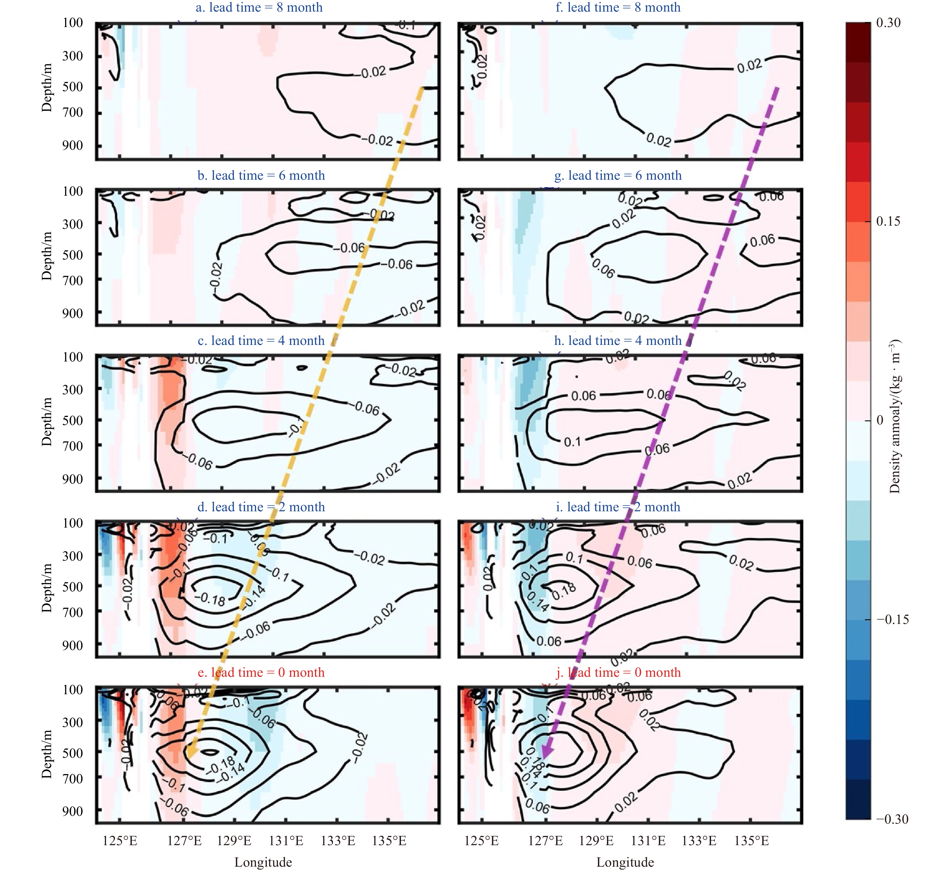
Figure 12 displays the vertical distribution of the westward propagating density anomaly signals, corresponding to those in Fig. 11, along the section shown in Fig. 11b. Similarly, the negative density anomaly signals occur 8 months before the strongest KGT (Fig. 12a). The subsurface core of the density anomaly is located at a depth of about 500 m. In the climatological mean state, the western boundary current maintains a horizontal density gradient with higher density on the left and lower density to the right, based on the thermal wind balance. Thus, when the negative density anomaly signals reach the offshore region of the RIC with a maximum core at about 128°E (Fig. 12c), they will strengthen the density gradient across the upstream Ryukyu Current, thereby enhancing its northward transport (about 127°E). Then, as the density anomaly signals continue to propagate westward, the negative density anomaly will enter the ECS and affect the region west of the RIC, thereby strengthening the density gradient and the northward flow of the upstream ECS-Kuroshio, which is located at about 126°E (Fig. 12e). Conversely, the positive density anomaly signals will relax the density gradient and decrease the upstream ECS-Kuroshio and Ryukyu Current (Figs 12f−j).

Figure  12.  Composite analysis of the vertical distribution of the density anomaly signals (contoured; unit: kg/m³) and the velocity anomalies (shaded; unit: m/s) perpendicular to the section shown in Fig. 11b, with time leads 8 months (a), 6 months (b), 4 months (c), 2 months (d), and 0 month (e) for the positive KGT year, 8 months (f), 6 months (g), 4 months (h), 2 months (i), and 0 month (j) for the negative KGT year. Ten yellow (purple) lines represent the propagation location of negative (postive) density anomaly signals.

DownLoad: Full-Size Img PowerPoint

5. Conclusions and discussion

This study uses monthly OFES data from 1950 to 2017 to investigate the interannual variability of volume transport through the Kerama Gap and its correlation with the Kuroshio/Ryukyu Current system. The surface geostrophic flow transport of different sections for the ECS-Kuroshio is compared with altimeter data, indicating that the OFES data are reliable in capturing the difference in interannual variability between the upstream and downstream transports of the ECS-Kuroshio separated by the Kerama Gap. The vertically integrated volume transport for both the ECS-Kuroshio and the Ryukyu Current also shows similar patterns of interannual variability. The interannual variability of the KGT shows a predominantly positive correlation with the upstream ECS-Kuroshio and Ryukyu Current and a predominantly negative correlation with the downstream Ryukyu Current, with all correlation coefficients exceeding 99% confidence level. The direction of the KGT changes with a mean volume transport of 0.6 × 10⁶ m³/s towards the Pacific Ocean and a higher standard deviation of 2.8 × 10⁶ m³/s. By comparing the standard deviation, the study finds that the interannual variability of the KGT is crucial for the differences between the upstream and downstream ECS-Kuroshio, while its contribution to the variability of the Ryukyu Current is relatively small, accounting for about 37%.

The study shows that the subsurface flow core located at 400–700 m is the main contributor to the interannual variability of the KGT, and such an interannual variability can be accurately reproduced by a two-layer rotating hydraulic theory. This theory demonstrated that the interannual variability of the KGT is mainly controlled by a subsurface pressure head, which forced by the interface height difference at 400 m between the two sides of the Kerama Gap. While the SSH difference makes a weak negative contribution to the interannual variation of KGT. Furthermore, the sensitivity experiments suggest that the interface height variability on the Pacific Ocean side is the key dynamic factor controlling the interannual variability of the KGT. While such interface height variability is mainly forced by the subsurface density anomalies, within a spatial region from 22°N to 26°N and 123°E to 132°E. These subsurface density anomaly signals originate in the interior of the Pacific Ocean and propagate westward at a speed of 7.4 km/d, consistent with the speed of the first-order baroclinic Rossby wave. When the core of the negative anomaly signals reaches the offshore region of the RIC and peaks 8 months later, it forms an anticyclonic vortex through baroclinic adjustment, leading to an increase in the upstream of the whole Kuroshio/Ryukyu Current system. Most of the additional upstream ECS-Kuroshio flows out of the ECS through the Kerama Gap. Meanwhile, the anticyclonic vortex generates an offshore current that runs parallel to the latitude of the Kerama Gap. As a compensating flow, the downstream Kuroshio is manifested as an anomalous southward flow, resulting in the negative correlation between the downstream Ryukyu Current and the KGT.

The model reveals that these processes are essentially two-layer baroclinic with subsurface intensification, and the interannual variability signals are also present at the sea surface. We therefore further validated the process using remote sensing SLA data. As illustrated in Fig. 13a, the altimeter effectively tracks the westward-propagating interannual variability signals along the same path as the density anomaly. The westward propagation speed of the SLA signals is about 7.9 km/d, consistent with the subsurface density anomaly signals of the model. Once the SLA signal reaches the southern side of the Kerama Gap, there are similar interannual variability can be found in surface geostrophic transport in both the Kerama Gap (Fig. 13b) and the upstream ECS-Kuroshio (Fig. 13c). The correlation coefficients between the SLA and these two transports are 0.56 and 0.60, respectively, both beyond the 99% level of significance. It proves that the dynamical mechanisms discovered in this work are robust.

Figure  13.  Time-dependent SLA during 1993–2017 along the path shown in Fig. 11a (a), interannual variability of the SLA at the westernmost point of the path (b), interannual variability of the SLD between the two endpoints of the section of the Kerama Gap (south minus north) (c), and interannual variability of the SLD between the two endpoints of the Section 5 of the ECS-Kuroshio (east minus west) (d).

DownLoad: Full-Size Img PowerPoint

It should be noted that not all the subsurface density anomaly signals to the south of the Kerama Gap originate from the east. Figure 14 provides an example of a positive density anomaly signal propagating southwest along the RIC into this region during April 1987 to February 1988, accompanied by a mesoscale cyclonic eddy. Further research is needed to determine the proportion of signals coming from the north and those coming from the east.

Figure  14.  A case analysis of the propagation of a positive density during April 1987 to February 1988. The vector represents the horizontal velocity and the shading represents the density anomaly at 500 m depth. The green line with stars represents the path followed to track the westward propagating density anomaly signals.

DownLoad: Full-Size Img PowerPoint