Yang Yingyi, Xu Tengfei, Wei Zexun, Wang Dingqi, Cai Zhongrui, Zhang Yunzhuo, Ma Yongshun. Interannual variability of surface Indonesian Throughflow and its relationships with Pacific and Indian Oceans derived from satellite observation[J]. Acta Oceanologica Sinica. doi: 10.1007/s13131-024-2396-6
Citation:
Yang Yingyi, Xu Tengfei, Wei Zexun, Wang Dingqi, Cai Zhongrui, Zhang Yunzhuo, Ma Yongshun. Interannual variability of surface Indonesian Throughflow and its relationships with Pacific and Indian Oceans derived from satellite observation[J]. Acta Oceanologica Sinica. doi: 10.1007/s13131-024-2396-6
Yang Yingyi, Xu Tengfei, Wei Zexun, Wang Dingqi, Cai Zhongrui, Zhang Yunzhuo, Ma Yongshun. Interannual variability of surface Indonesian Throughflow and its relationships with Pacific and Indian Oceans derived from satellite observation[J]. Acta Oceanologica Sinica. doi: 10.1007/s13131-024-2396-6
Citation:
Yang Yingyi, Xu Tengfei, Wei Zexun, Wang Dingqi, Cai Zhongrui, Zhang Yunzhuo, Ma Yongshun. Interannual variability of surface Indonesian Throughflow and its relationships with Pacific and Indian Oceans derived from satellite observation[J]. Acta Oceanologica Sinica. doi: 10.1007/s13131-024-2396-6
First Institute of Oceanography, and Key Laboratory of Marine Science and Numerical Modeling, Ministry of Natural Resources, Qingdao 266061, China
2.
Laboratory for Regional Oceanography and Numerical Modeling, Qingdao Marine Science and Technology Center, Qingdao, 266237, China
3.
Shandong Key Laboratory of Marine Science and Numerical Modeling, Qingdao 266061, China
4.
CMA-NJU Joint Laboratory for Climate Prediction Studies, School of Atmospheric Sciences, Nanjing University, Nanjing, China
5.
Earth, Ocean and Atmospheric Sciences Thrust, The Hong Kong University of Science and Technology (Guangzhou), Guangzhou 511400, China
6.
Zhonghai Yuntian (Guangdong) Marine Technology Co., LTD, Guangzhou 510275, China
Funds:
The Fund of Laoshan Laboratory under contract No. LSKJ202202700; the Basic Scientific Fund for National Public Research Institutes of China (2024Q02); the National Natural Science Foundation of China under grant Nos. 42076023 and 42430402; the Global Change and Air-Sea Interaction II Project under contract No. GASI-01-AIP-STwin
The Indonesian Throughflow (ITF) plays important roles in global ocean circulation and climate systems. Previous studies suggested the ITF interannual variability is driven by both the El Niño-Southern Oscillation (ENSO) and the Indian Ocean Dipole (IOD) events. The detailed processes of ENSO and/or IOD induced anomalies impacting on the ITF, however, are still not clear. In this study, this issue is investigated through causal relation, statistical and dynamical analyses based on satellite observation. The results show that the driven mechanisms of ENSO on the ITF include two aspects. Firstly, the ENSO related wind field anomalies driven anomalous cyclonic ocean circulation in the western Pacific, and off equatorial upwelling Rossby waves propagating westward to arrive at the western boundary of the Pacific, both tend to induce negative sea surface height anomalies (SSHA) in the western Pacific, favoring ITF reduction since the develop of the El Niño through the following year. Secondly, the ENSO events modulate equatorial Indian Ocean zonal winds through Walker Circulation, which in turn trigger eastward propagating upwelling Kelvin waves and westward propagating downwelling Rossby waves. The Rossby waves are reflected into downwelling Kelvin waves, which then propagate eastward along the equator and the Sumatra-Java coast in the Indian Ocean. As a result, the wave dynamics tend to generate negative (positive) SSHA in the eastern Indian Ocean, and thus enhance (reduce) the ITF transport with time lag of 0–6 (9–12) month, respectively. Under the IOD condition, the wave dynamics also tend to enhance the ITF in the positive IOD year, and reduce the ITF in the following year.
Figure 1. Annual mean sea surface currents (vector) and SSHA (shaded) in the western Pacific and eastern Indian Oceans. Sections for surface transport calculation are NEC: 8°–18°N, 130°E; MC: 8°N, 126°–130°E; KC: 18°N, 122.25°–130°E; IX1: 26°S, 113.76°E–4.95°S, 104.32°E.
Figure 2. (a) Hovmöller plot of zonal velocity along the IX1 section; (b) TITF and the Latu=0 in the IX1 section; (c) surface transport anomalies of the Pacific NEC, MC, KC, and the ITF; (d) NECBL anomalies (solid line) and ITF southernmost boundary latitude (Latu=0) anomalies (dashed line).
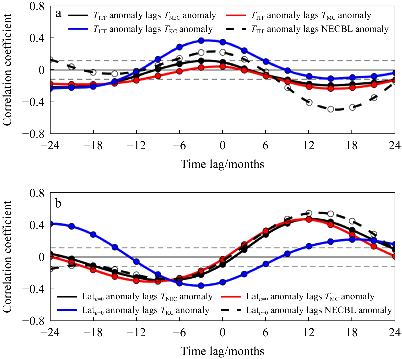
Figure 3. Lag correlations of (a) TITF anomalies with TNEC (black solid line), TMC (red solid line), TKC (blue solid line), and NECBL anomalies (black dashed line); (b) Latu=0 anomalies with TNEC (black solid line), TMC (red solid line), TKC (blue solid line), and NECBL anomalies (black dashed line). Positive/negative months on the x-axes indicate TITF and Latu=0 anomalies lagging/leading the other anomalies; and dashed horizontal lines stand for the 95% significance level.
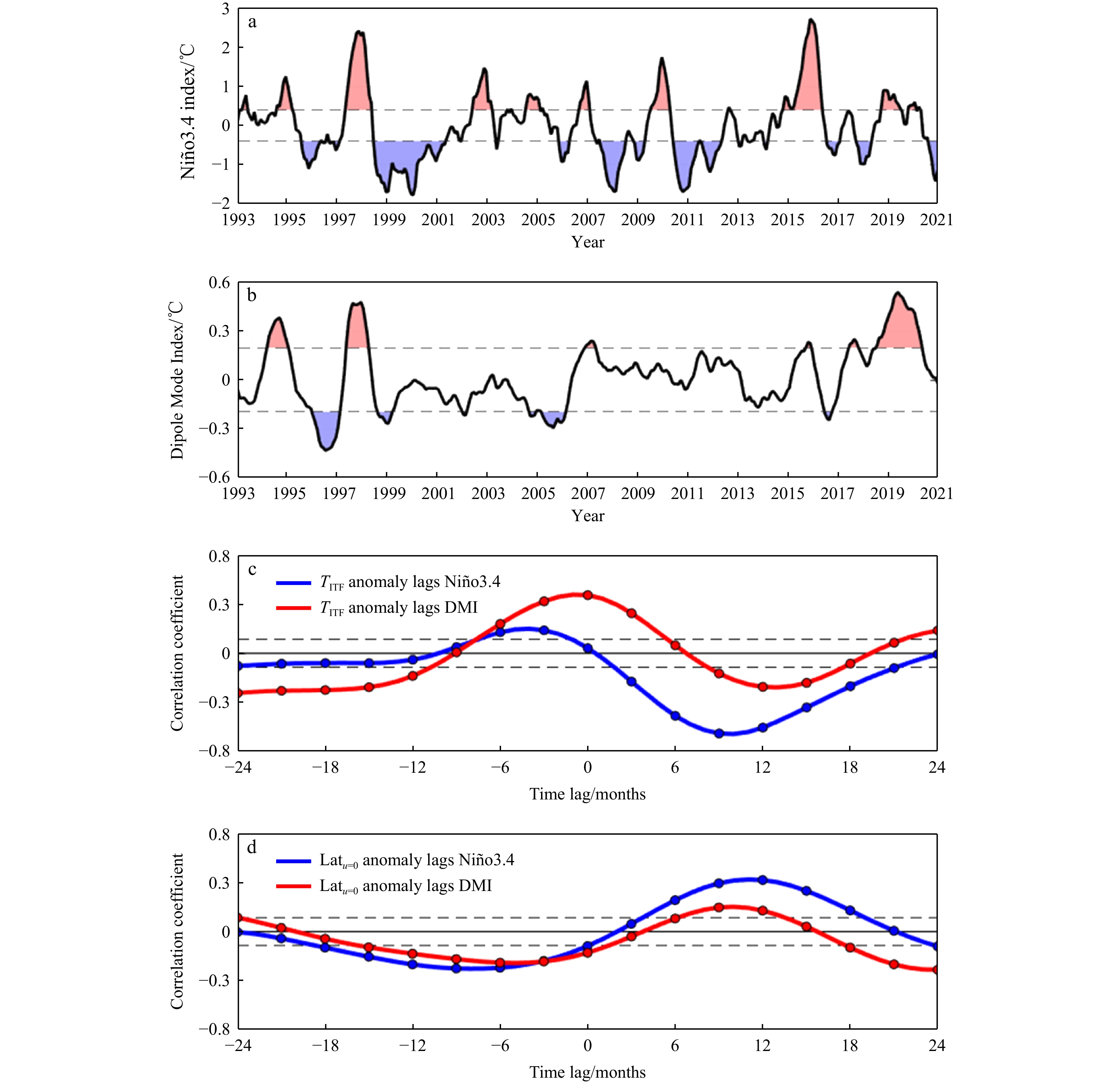
Figure 4. (a) Niño3.4, and (b) DMI indices; lag correlations of (c) TITF and (d) Latu=0 anomalies with Niño3.4 (blue line) and DMI (red line) indices. Positive months indicate that Indo-Pacific climate indices lead ITF variability. Dashed line stands for the 95% confidence level.
Figure 5. Composite (a) TITF and (b) Latu=0 anomalies for El Niño, La Niña, pIOD, and El Niño-pIOD, La Niña-nIOD co-occurred events.
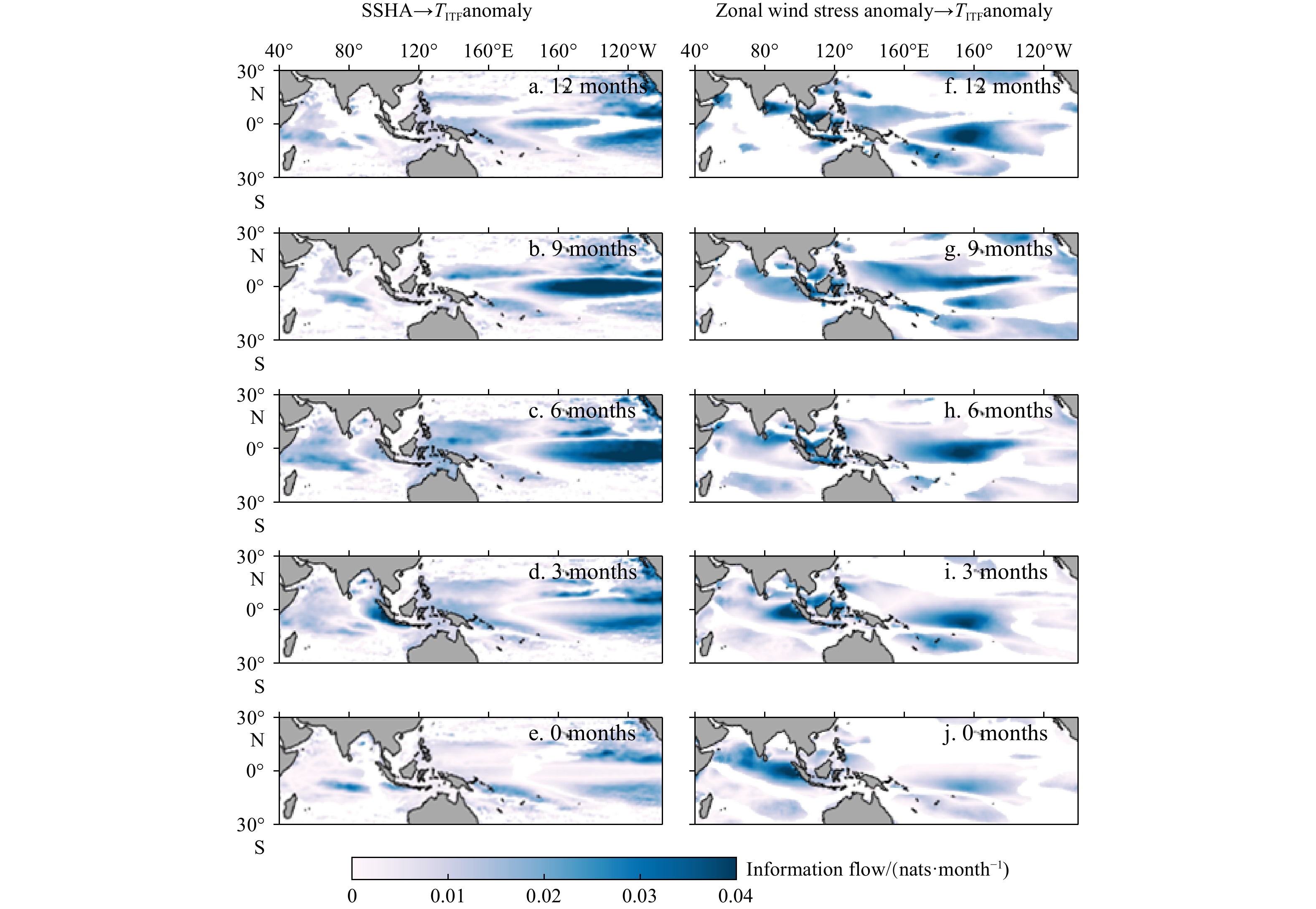
Figure 6. (a)–(e) Absolute information flow from SSHA in the tropical Indo-Pacific Ocean to TITF anomalies, with the later lagging by 12–0 months; (f)–(j) same as (a)–(e), but from ZWSA to TITF anomalies. Shadings indicate those above the 95% significance level.
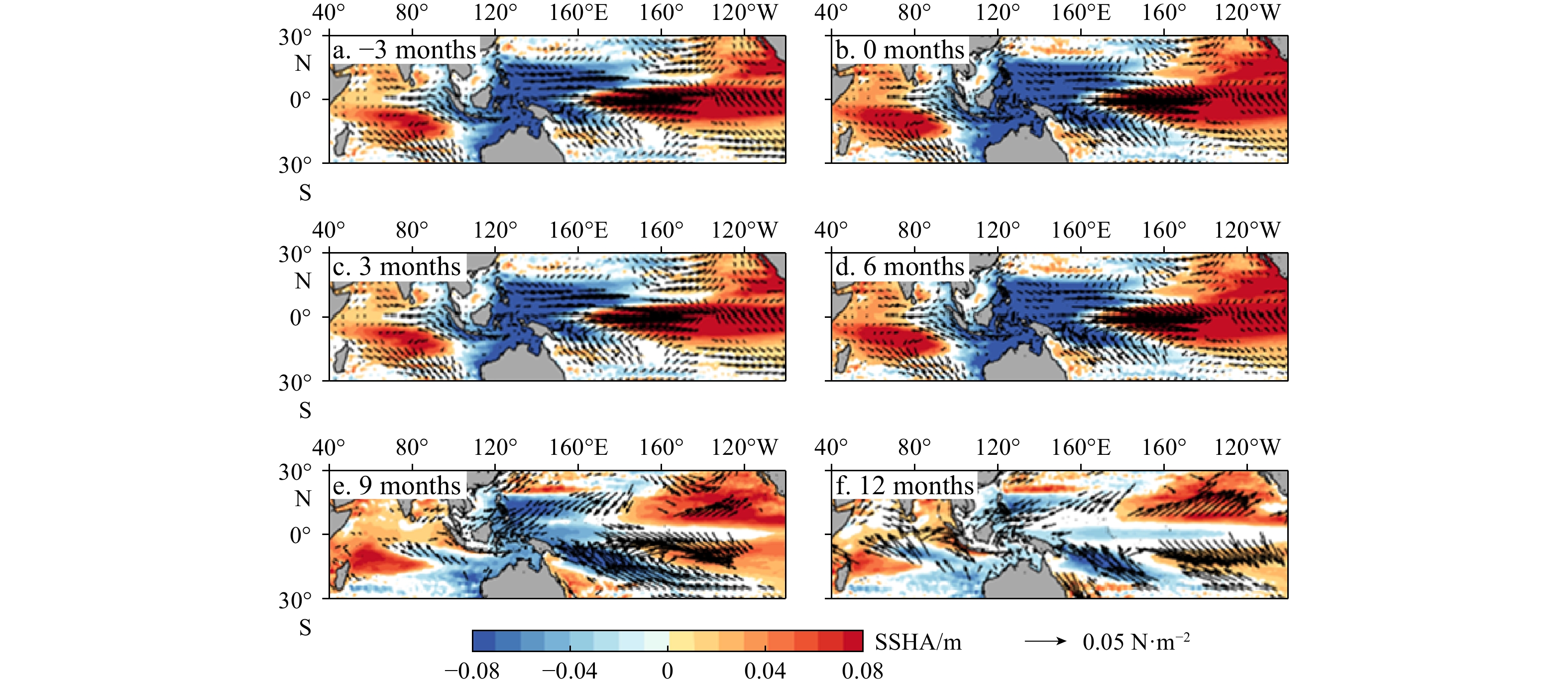
Figure 7. SSHA (shading) and wind stress anomalies (vector) regressed on Niño3.4 indices, with (a) leading time of 3 months, (b) synchronous regression, and (c)–(f) lagging time of 3–12 months. Only values above the 95% significance level are shown.
Figure 8. SSHA (shading) and wind stress anomalies (vector) regressed on DMI indices, with (a) leading time of 3 months, (b) synchronous regression, and (c)–(f) lagging time of 3–12 months. Only values above the 95% significance level are shown.
Figure 9. (a) Hovmöller diagram of wind stress (vector) and wind stress curl (shading) anomalies averaged between 12°–14°N in the Pacific Ocean; (b) same as (a), but for SSHA; (c) time series of TITF; (d) and (e) are same as (a) and (b), but averaged between 2°N–2°S in the Indian Ocean.
Figure 10. (a) Time series of area averaged SSHA (2°N–2°S, 98°–100°E); (b)–(j) composite SSHA (shading) and sea surface wind anomalies (vector) in the tropical Indian Ocean from month -1 to month +7, with month 0 refer to as the peak of the selected negative SSHA events as shown in (a).
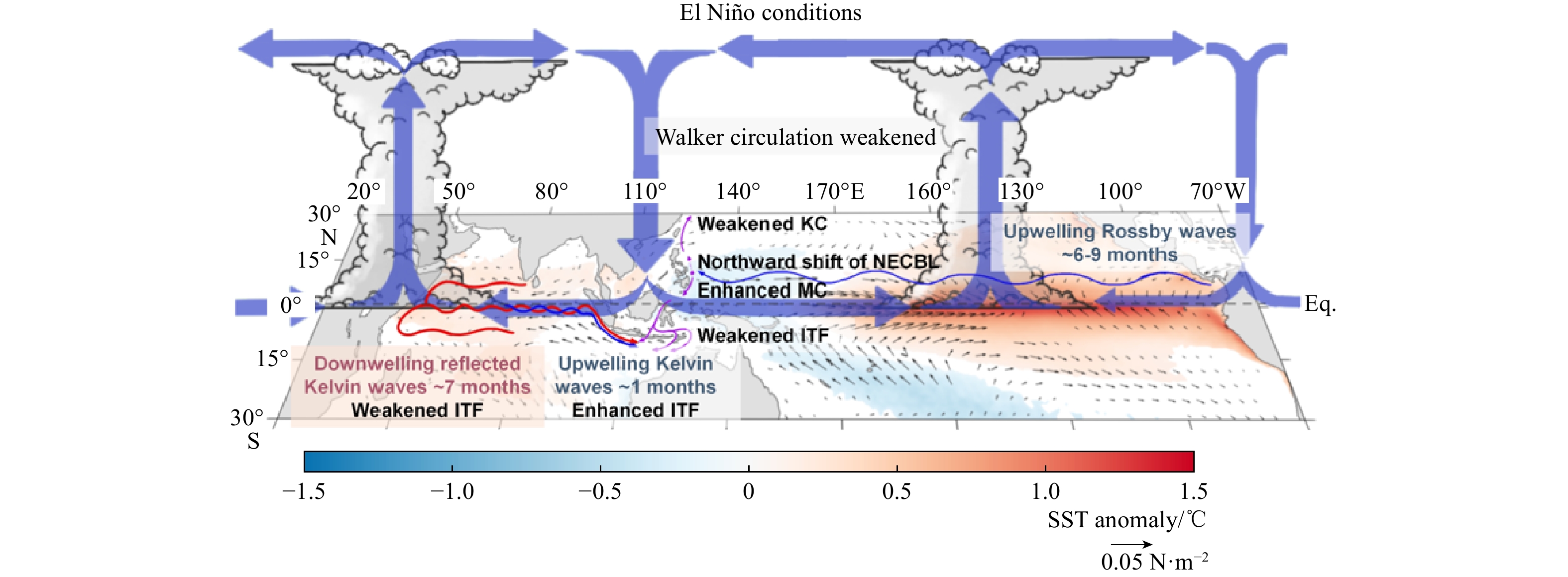
Figure 11. Schematic of the ITF in response to the El Niño condition. SST (shading) and wind stress anomalies (vector) regressed on Niño3.4 indices.
Figure 12. Schematic of the ITF in response to the positive IOD condition. SST (shading) and wind stress anomalies (vector) regressed on DMI indices: (a) synchronous regression and (b) lagging time of 12 months.


 DownLoad: