

Principal-component estimates of the Kuroshio Current axis and path based on the mathematical verification between satellite altimeter and drifting buoy data
-
Abstract: We used satellite altimetry data to investigate the Kuroshio Current because of the higher resolution and wider range of observations. In previous studies, satellite absolute geostrophic velocities were used to study the spatio-temporal variability of the sea surface velocity field along the current, and extraction methods were employed to detect the Kuroshio axes and paths. However, sea surface absolute geostrophic velocity estimated from absolute dynamic topography should be regarded as the geostrophic component of the actual surface velocity, which cannot represent a sea surface current accurately. In this study, mathematical verification between the climatic absolute geostrophic and bin-averaged drifting buoy velocity was established and then adopted to correct the satellite absolute geostrophic velocities. There were some differences in the characteristics between satellite geostrophic and drifting buoy velocities. As a result, the corrected satellite absolute geostrophic velocities were used to detect the Kuroshio axis and path based on a principal-component detection scheme. The results showed that the detection of the Kuroshio axes and paths from corrected absolute geostrophic velocities performed better than those from satellite absolute geostrophic velocities and surface current estimations. The corrected satellite absolute geostrophic velocity may therefore contribute to more precise day-to-day detection of the Kuroshio Current axis and path.
-
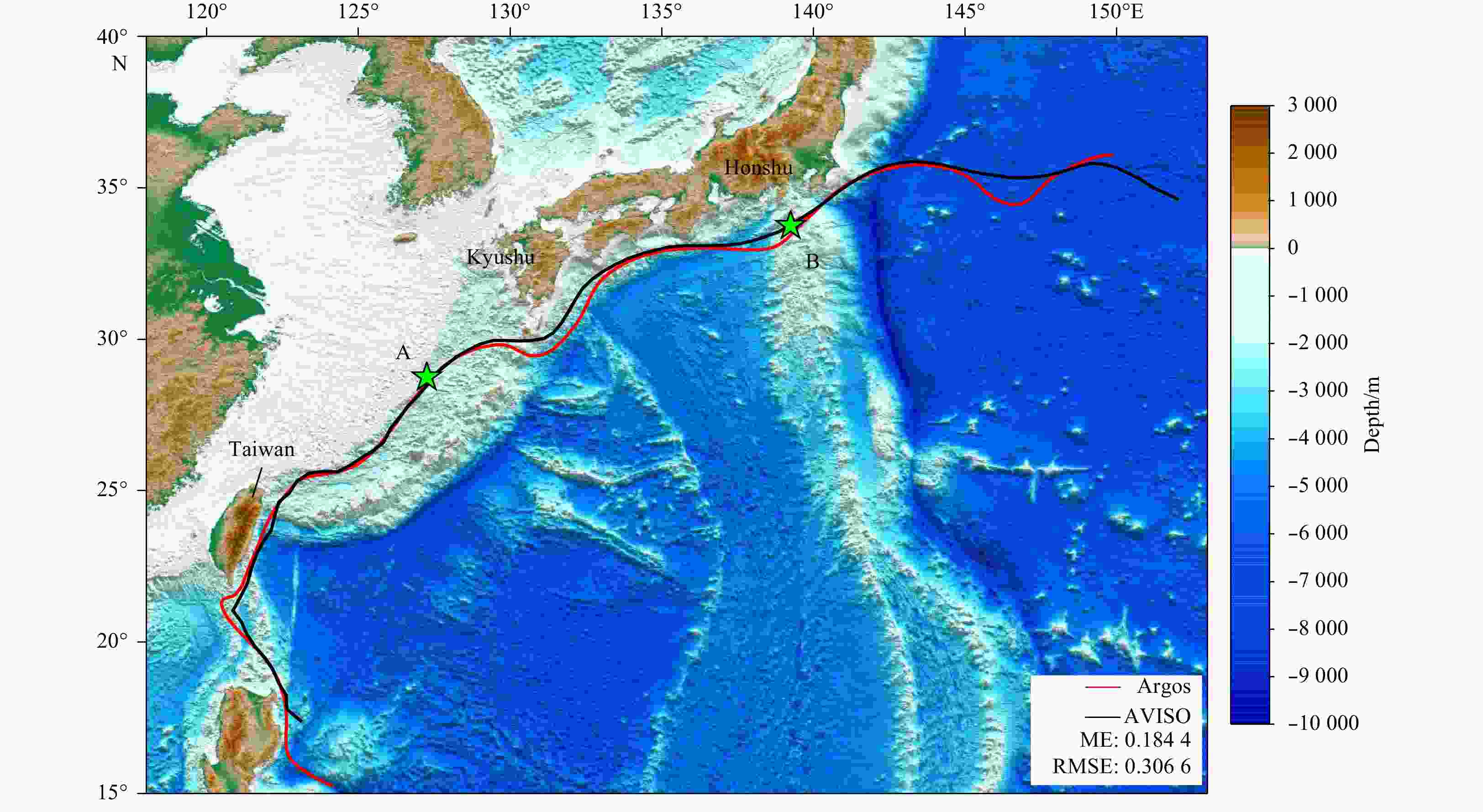
Figure 1. The study region with bathymetry. Climatic information of the Kuroshio Current is derived from the yearly averaged results from 1993–2017 merged with absolute geostrophic (blue line) and 38 a (1979–2016) Argos drifting buoy (red line) velocities. The mean error (ME) and root mean square error (RMSE) between these two lines were calculated. Two representative points (green stars), located at 28.75°N, 127.25°E (Point A) and 33.75°N,139.25°E (Point B), were chosen to show the fitting functions at the coefficient grids. The scatter diagrams are shown in Fig. 4.

Figure 2. Distribution diagram of the data and coefficient grids. The red points denote the centers of the data grids and the black crosses indicate the coefficient grid centers represented as black solid lines.
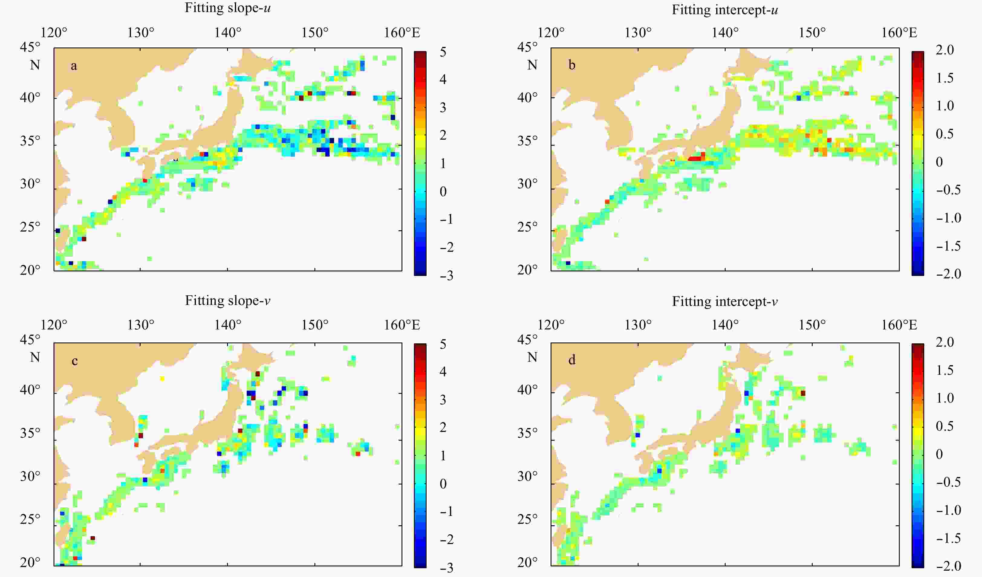
Figure 5. Spatial distribution of the Kuroshio Current velocities linear relationship, including the slope (a, c) and intercept (b, d), of the fitting lines. a and b denote the zonal components of the velocities while b and d indicate the meridional components. The blank regions (white areas) represent areas where the mathematical relationship could not be established.
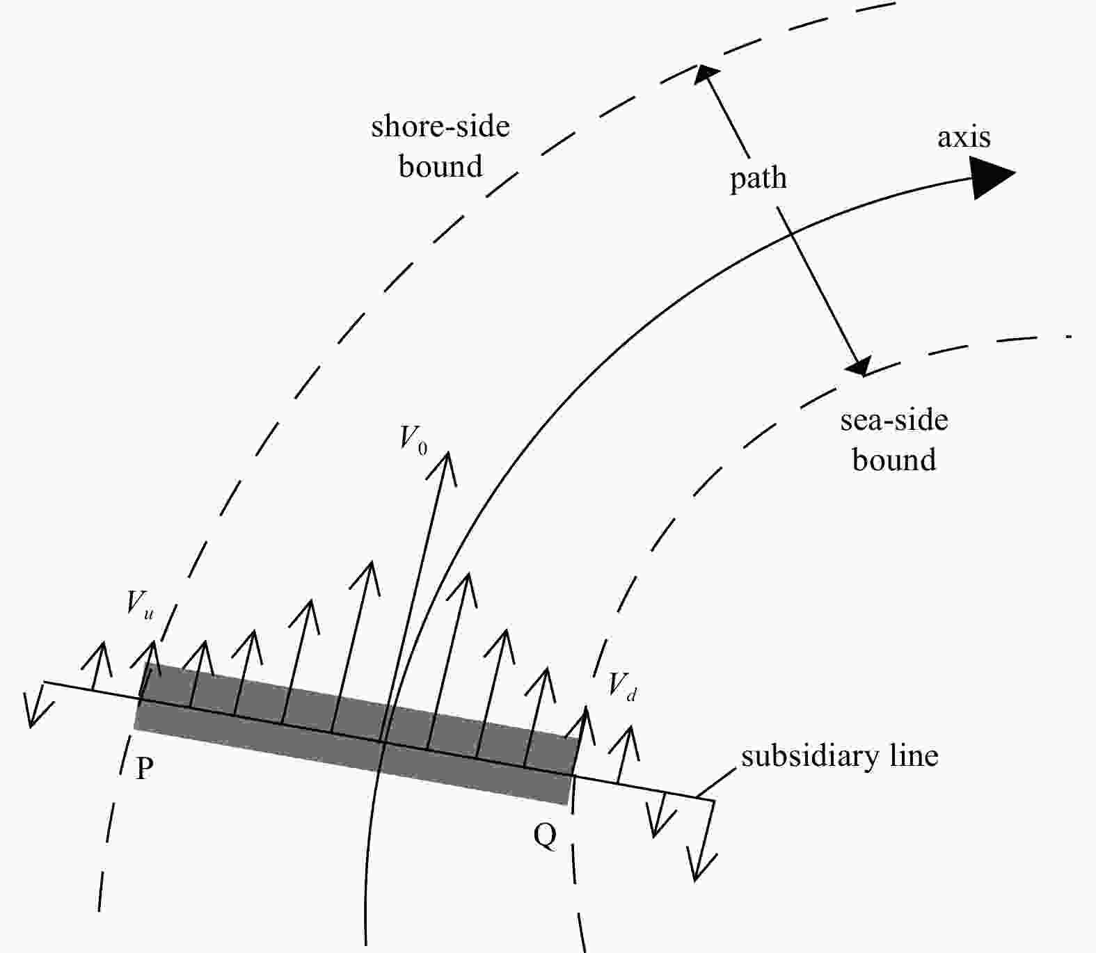
Figure 3. Schematic of the axis, shore-side and sea-side boundaries, subsidiary line, maximum velocity at the axis (V0) and boundary velocities (Vu and Vd).
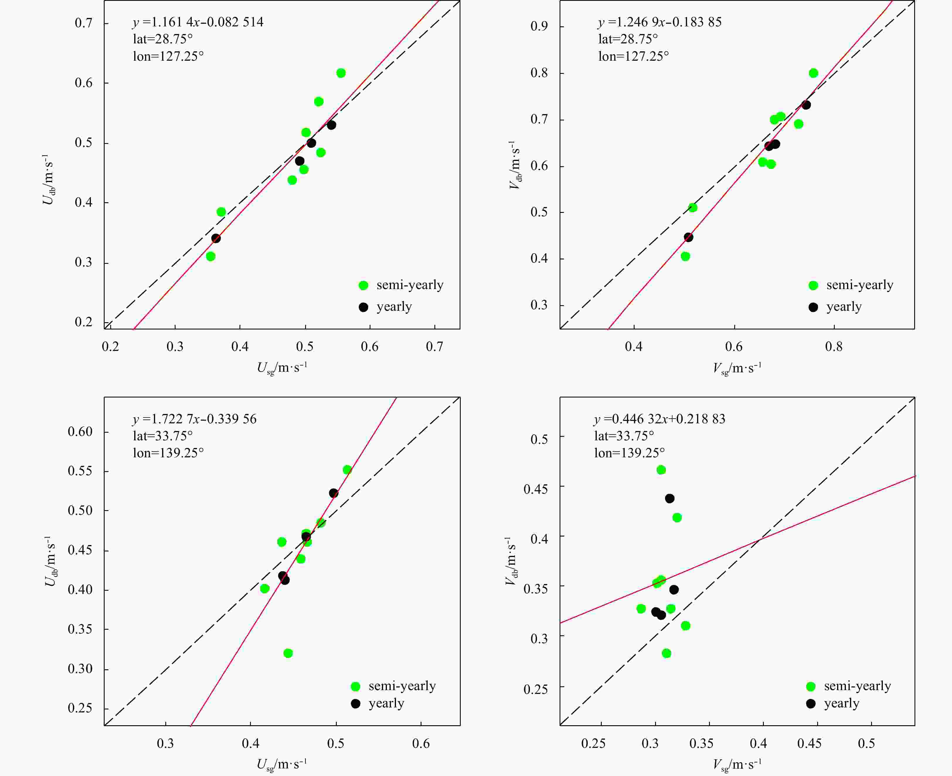
Figure 4. Scatter diagrams of the satellite geostrophic velocities versus drifting buoy velocities, including zonal component U (left panels) and meridional component V (right panels); the red solid lines indicate the linear relationship between the two results. As a reference, the black dashed lines denote standard lines corresponding to y=x. In the top left portions of each panel, the linear relationship equation is shown along with the longitude and latitude corresponding to the center of the (1/2)° × (1/2)° coefficient grids.
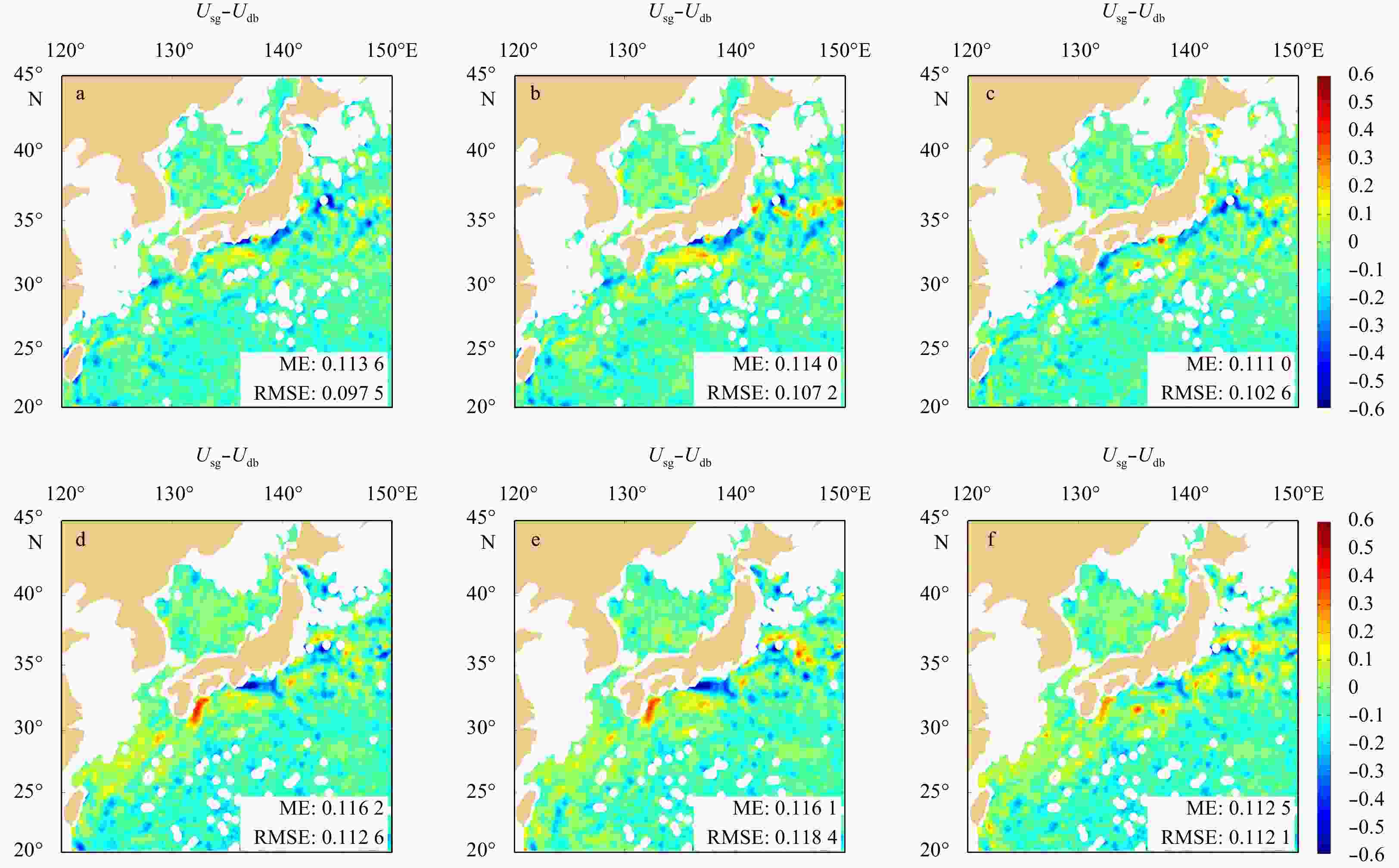
Figure 6. Difference of the surface velocity fields (m/s) calculated by subtracting the satellite geostrophic (Usg) and corrected satellite geostrophic (Uag) velocities and surface current estimates (Use) from the bin-averaged drifting buoy velocities (Udb). The mean error (ME, m/s) and root mean square error (RMSE, m/s) are shown. The top and bottom panels correspond to the summer and winter seasonal averaged results, respectively. The blank regions (white areas) correspond to the invalid grids of the Udb fields.
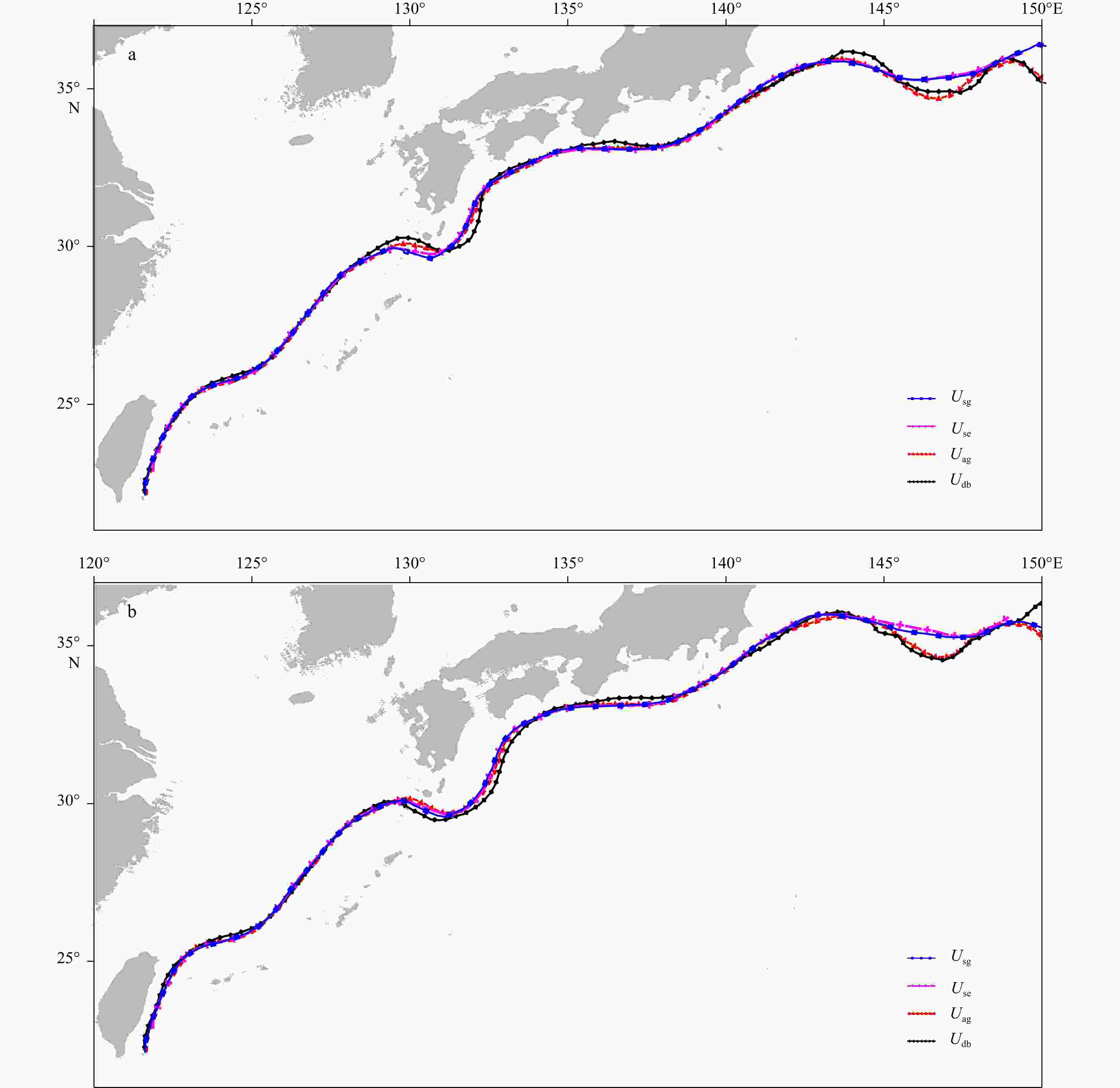
Figure 7. Distribution of the seasonal averaged locations of the Kuroshio Current axes in (a) summer and (b) winter based on four different surface velocity fields, including satellite absolute geostrophic velocities (AGVs, blue line with solid symbols), surface current estimates (magenta line with cross symbols), corrected satellite AGVs (red line with triangle symbols) and the bin-averaged drifting buoy velocities (DBVs, black line with diamond symbols).
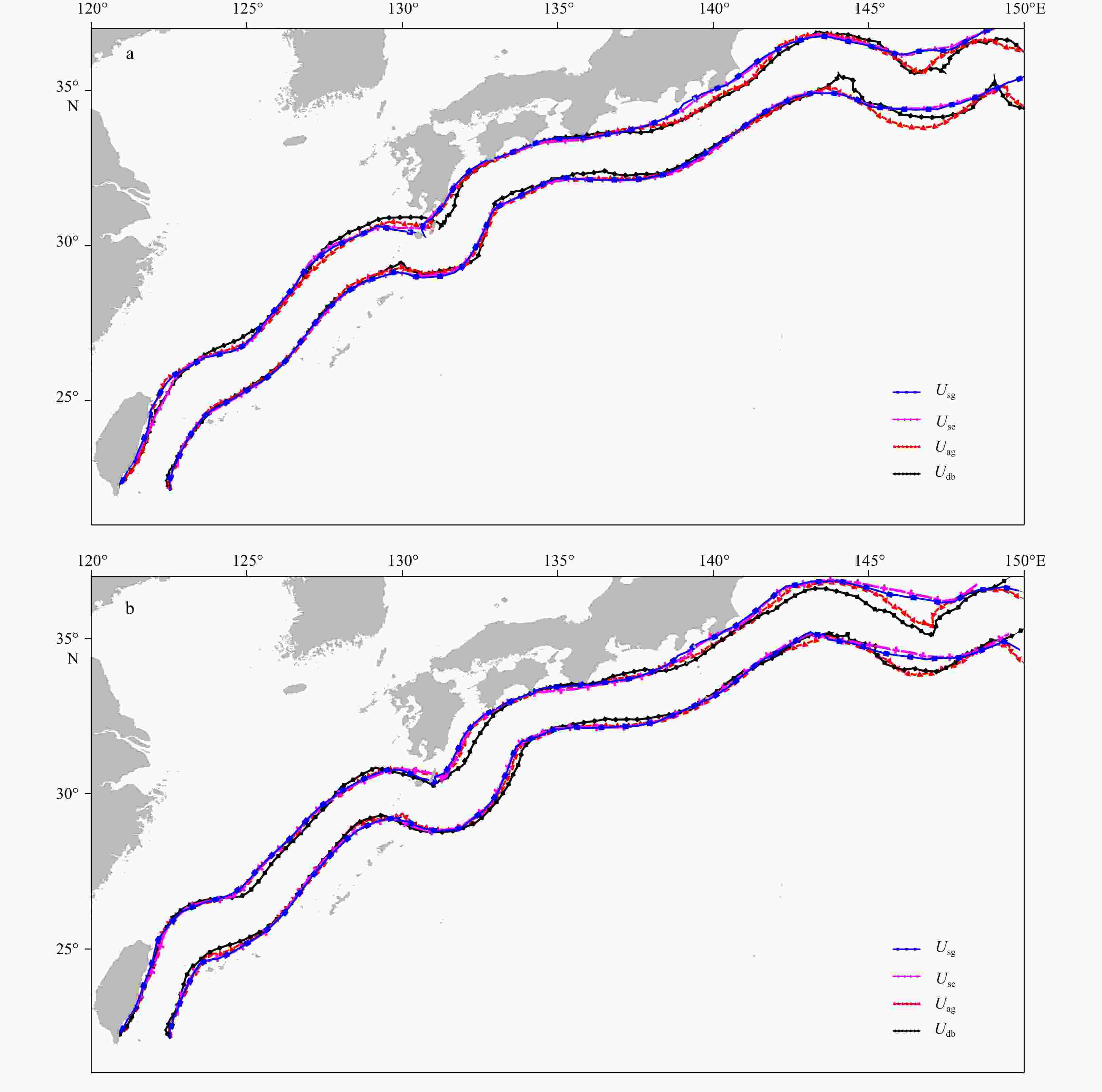
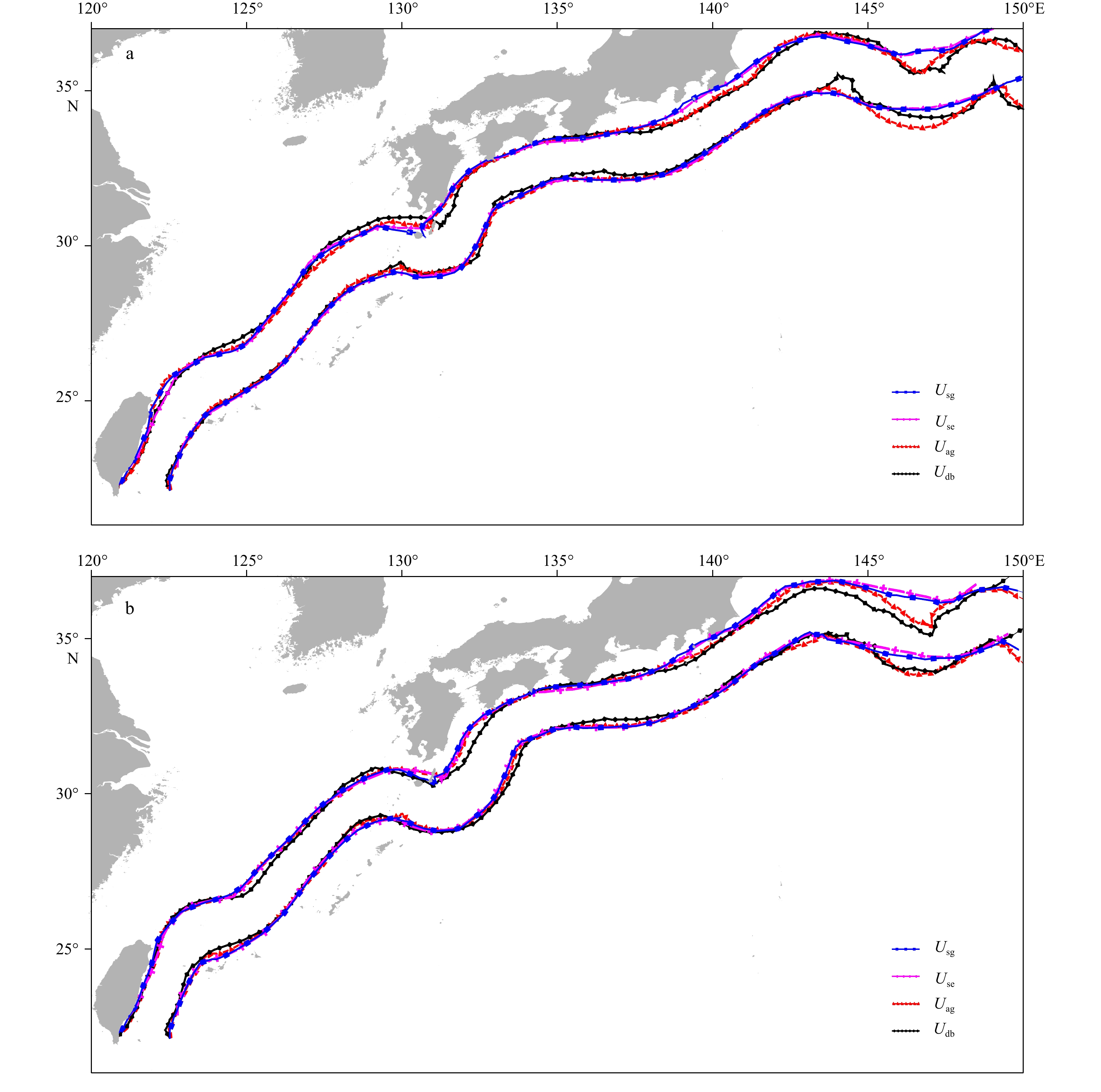
Figure 8. Distribution of the seasonal averaged locations of the Kuroshio Current paths in summer (a) and winter (b) based on four different surface velocity fields, including satellite absolute geostrophic velocities (AGVs, blue line with solid symbols), surface current estimates (magenta line with cross symbols), corrected satellite AGVs (red line with triangle symbols) and the bin-averaged drifting buoy velocities (DBVs, black line with diamond symbols).
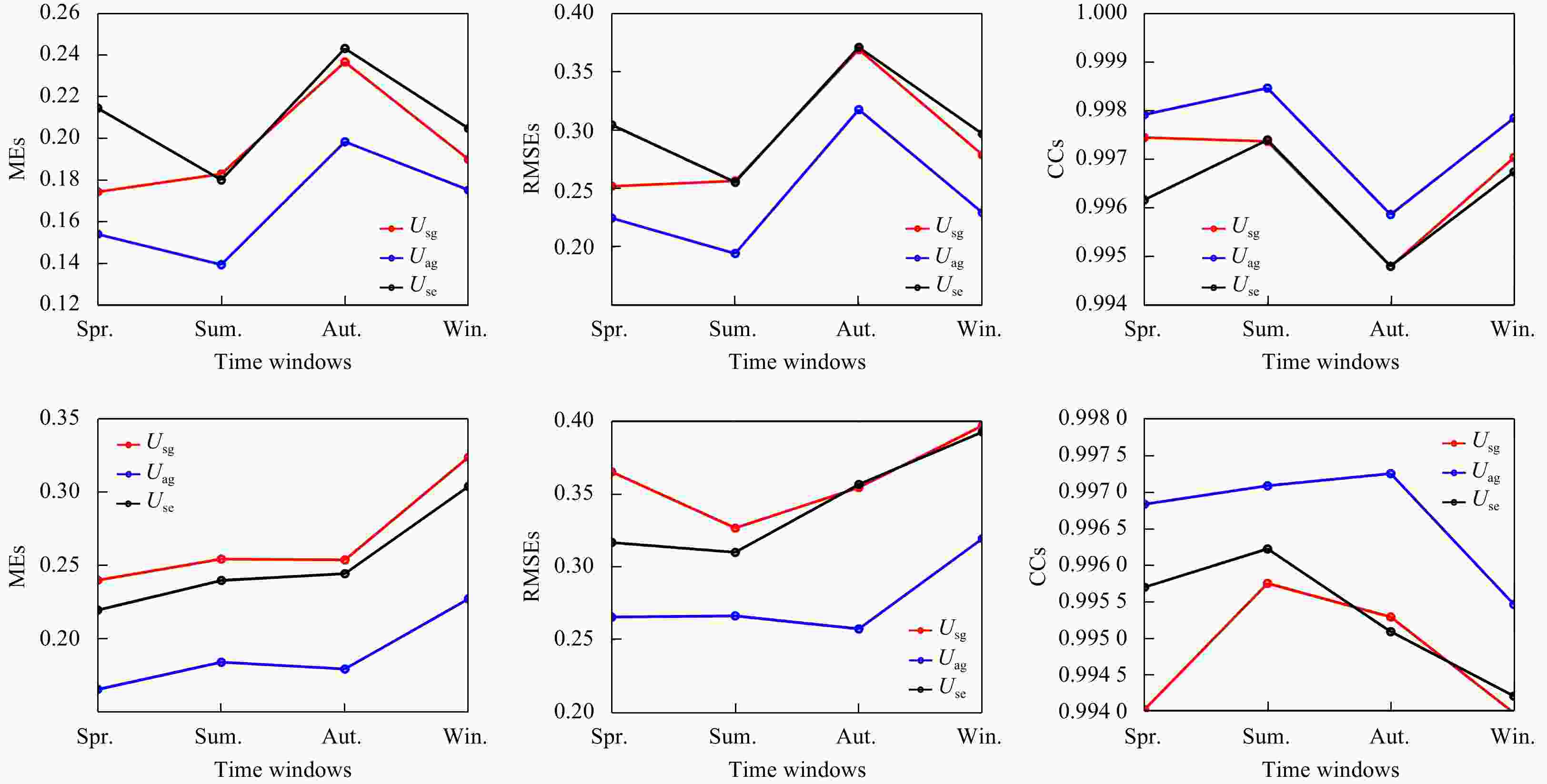
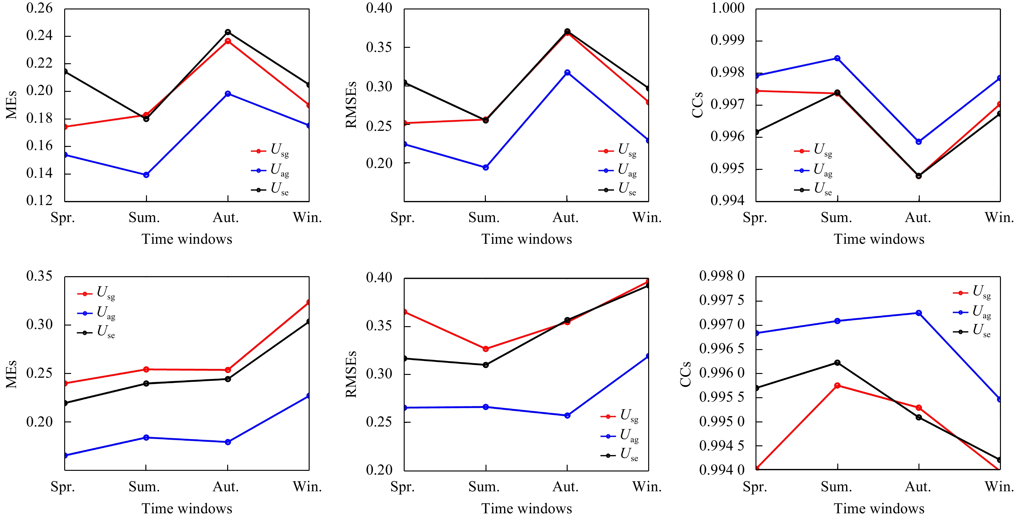
Figure 9. The mean errors (MEs, left panels), root mean square errors (RMSEs, middle panels) and correlation coefficients (CCs, right panels) of the detected KC axes (first row) and paths (second row) were calculated between Usg and Udb (red lines), Uag and Udb (blue lines), and Use and Udb (black lines) corresponding to four seasonal averaged results, including spring (Spr.), summer (Sum.), autumn (Aut.) and winter (Win.).
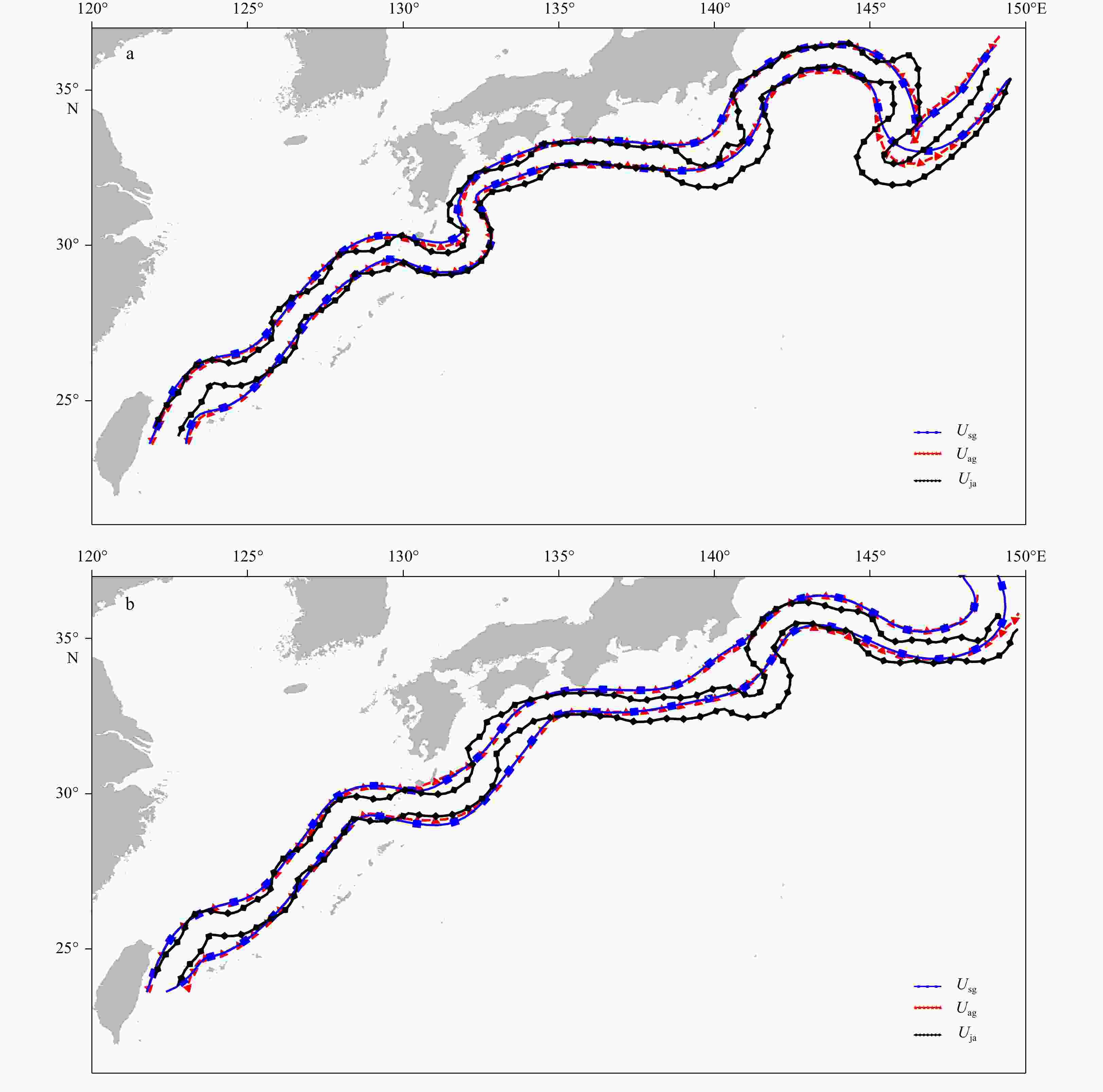
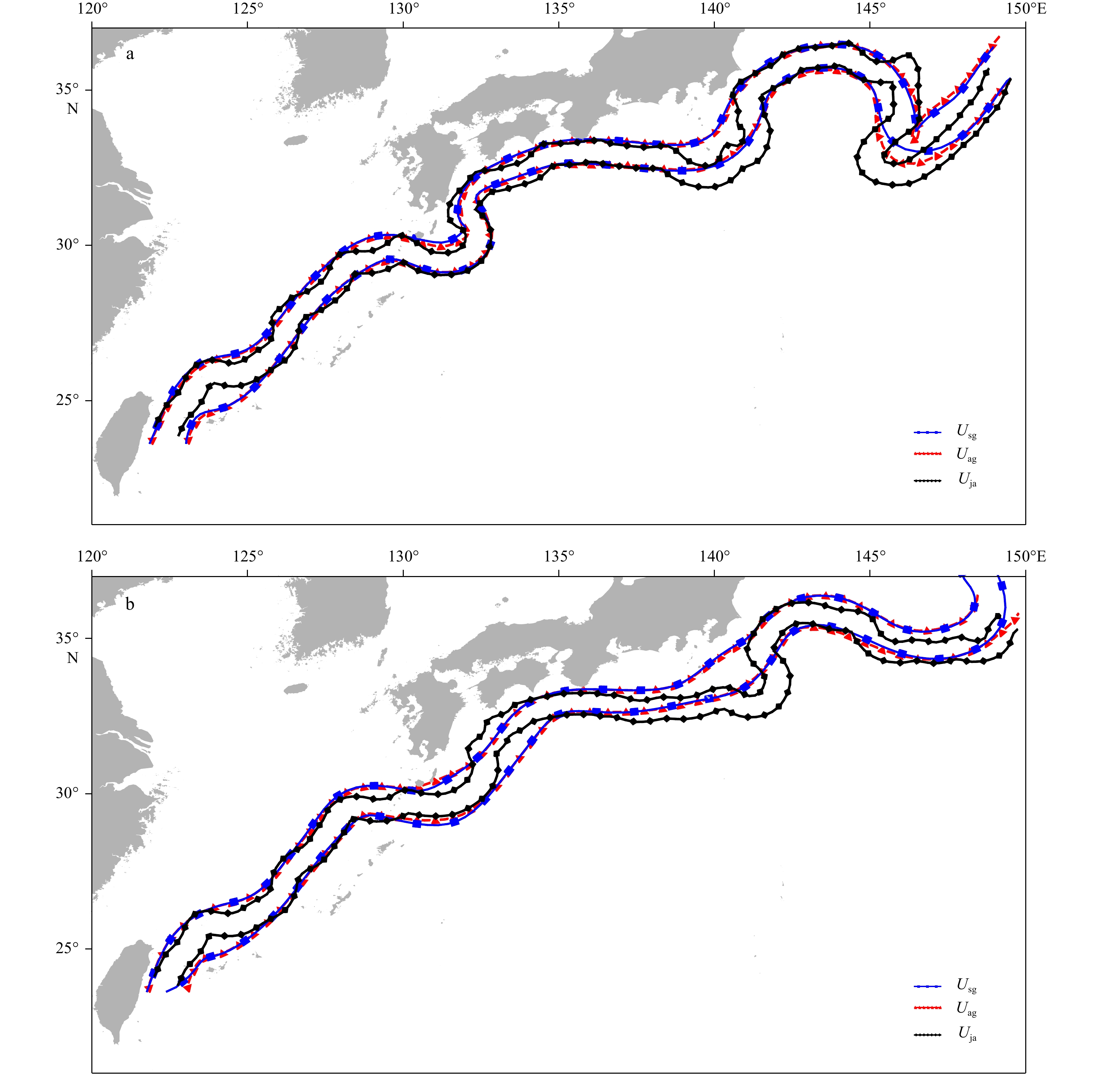
Figure 10. Distribution of the Kuroshio Current paths on 4 January 2018 (a) and 20 January 2018 (b) based on satellite AGVs (blue line with square symbols), corrected satellite AGVs (red line with triangle symbols) and daily current maps (black line with diamond symbols).
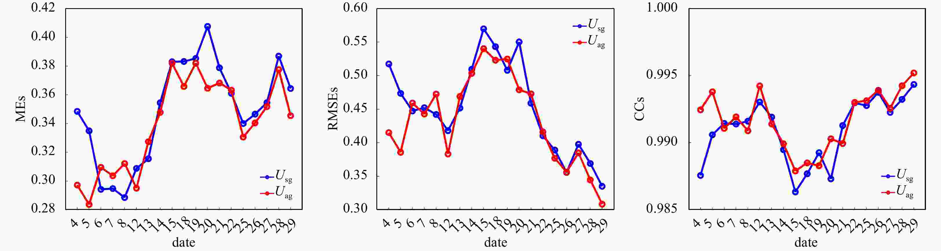
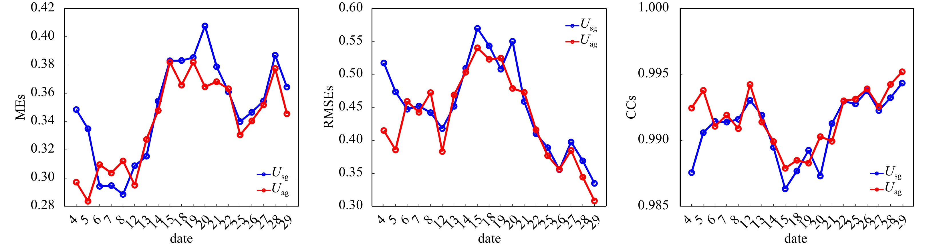
Figure 11. The mean errors (MEs, left panels), root mean square errors (RMSEs, middle panels) and correlation coefficients (CCs, right panels) of the Kuroshio Current path locations. These indices calculated between Usg and Uja (red lines) and Uag and Uja (blue lines) in January 2018. All the days of January which is recorded in quick report maps from HOD are selected.
-
[1] Ambe D, Imawaki S, Uchida H, et al. 2004. Estimating the Kuroshio Axis South of Japan using combination of satellite altimetry and drifting buoys. Journal of Oceanography, 60(2): 375–382. doi: 10.1023/B:JOCE.0000038343.31468.fe [2] Arbic B K, Scott R B, Chelton D B, et al. 2012. Effects of stencil width on surface ocean geostrophic velocity and vorticity estimation from gridded satellite altimeter data. Journal of Geophysical Research: Oceans, 117(C3): C03029. doi: 10.1029/2011JC007367 [3] CNES. 2016. SSALTO/DUACS User Handbook: (M)SLA and (M)ADT Near-Real Time and Delayed Time Products. CLS-DOS-NT-06-034 [4] Hu Xiaomin, Xiong Xuejun, Qiao Fangli, et al. 2008. Surface current field and seasonal variability in the Kuroshio and adjacent regions derived from satellite-tracked drifter data. Acta Oceanologica Sinica, 27(3): 11–29 [5] Hui Zhenli, Xu Yongsheng. 2016. The impact of wave-induced Coriolis-Stokes forcing on satellite-derived ocean surface currents. Journal of Geophysical Research: Oceans, 121(1): 410–426. doi: 10.1002/2015JC011082 [6] Imawaki S, Gotoh M, Yoritaka H, et al. 1996. Detecting fluctuations of the Kuroshio axis south of Japan using TOPEX/POSEIDON altimeter data. Journal of Oceanography, 52(1): 69–92. doi: 10.1007/BF02236533 [7] Ishikawa Y, Awaji T, Akimoto K. 1997. Global surface circulation and its kinetic energy distribution derived from drifting buoys. Journal of Oceanography, 53(5): 489–516 [8] Lagerloef G S E, Mitchum G T, Lukas R B, et al. 1999. Tropical Pacific near-surface currents estimated from altimeter, wind, and drifter data. Journal of Geophysical Research: Oceans, 104(C10): 23313–23326. doi: 10.1029/1999JC900197 [9] Liu Zhiqiang, Gan Jianping. 2012. Variability of the Kuroshio in the East China Sea derived from satellite altimetry data. Deep Sea Research Part I: Oceanographic Research Papers, 2012, 59: 25–36 [10] Matsuno T, Lee J S, Yanao S. 2009. The Kuroshio exchange with the South and East China Seas. Ocean Science, 5: 303–312. doi: 10.5194/os-5-303-2009 [11] Miyazawa Y, Kagimoto T, Guo X Y, et al. 2008. The Kuroshio large meander formation in 2004 analyzed by an eddy-resolving ocean forecast system. Journal of Geophysical Research: Oceans, 113(C10): C10015. doi: 10.1029/2007JC004226 [12] Philipps O M. 1977. The Dynamics of the Upper Ocean. Cambridge, UK: Cambridge University Press [13] Qiu Bo. 2001. Kuroshio and Oyashio currents. In: Steele J H, Turekian K K, eds. Encyclopedia of Ocean Sciences. New York: Elsevier, 1413–1425 [14] Teague W J, Jacobs G A, Ko D S, et al. 2003. Connectivity of the Taiwan, Cheju, and Korea straits. Continental Shelf Research, 23(1): 63–77. doi: 10.1016/S0278-4343(02)00150-4 [15] Uchida H, Imawaki S. 2003. Eulerian mean surface velocity field derived by combining drifter and satellite altimeter data. Geophysical Research Letters, 30(5): 1229. doi: 10.1029/2002GL016445 [16] Wu Kejian, Liu Bin. 2008. Stokes drift-induced and direct wind energy inputs into the Ekman layer within the Antarctic Circumpolar Current. Journal of Geophysical Research: Oceans, 113(C10): C10002. doi: 10.1029/2007JC004579 -

 下载:
下载:


 点击查看大图

计量
- 文章访问数: 714
- HTML全文浏览量: 201
- PDF下载量: 116
- 被引次数: 0