

An improved optical flow method to estimate Arctic sea ice velocity (winter 2014−2016)
-
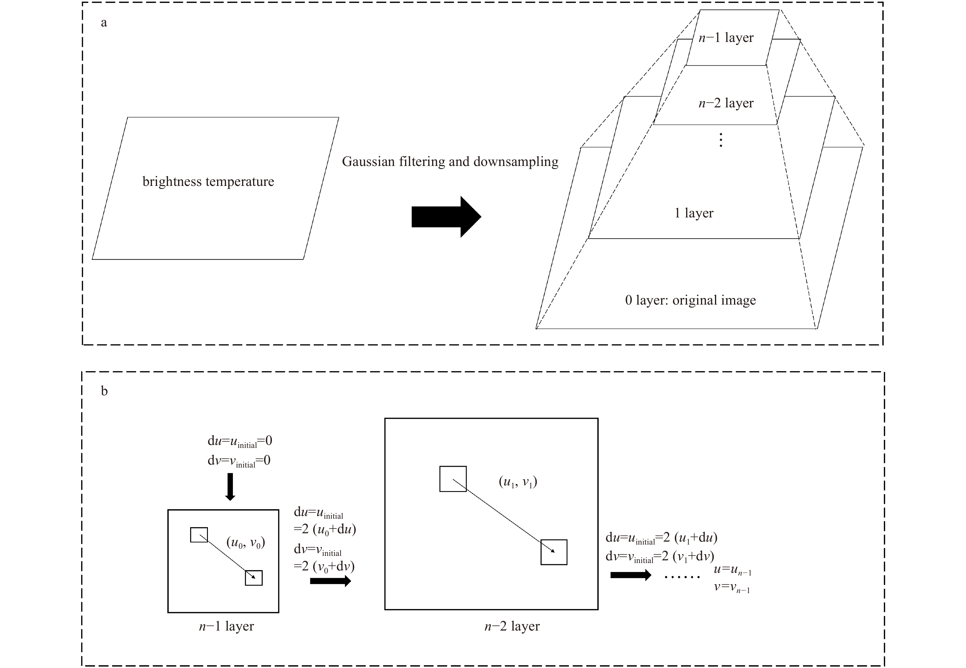
Abstract: Sea ice velocity impacts the distribution of sea ice, and the flux of exported sea ice through the Fram Strait increases with increasing ice velocity. Therefore, improving the accuracy of estimates of the sea ice velocity is important. We introduce a pyramid algorithm into the Horn-Schunck optical flow (HS-OF) method (to develop the PHS-OF method). Before calculating the sea ice velocity, we generate multilayer pyramid images from an original brightness temperature image. Then, the sea ice velocity of the pyramid layer is calculated, and the ice velocity in the original image is calculated by layer iteration. Winter Arctic sea ice velocities from 2014 to 2016 are obtained and used to discuss the accuracy of the HS-OF method and PHS-OF (specifically the 2-layer PHS-OF (2LPHS-OF) and 4-layer PHS-OF (4LPHS-OF)) methods. The results prove that the PHS-OF method indeed improves the accuracy of sea ice velocity estimates, and the 2LPHS-OF scheme is more appropriate for estimating ice velocity. The error is smaller for the 2LPHS-OF velocity estimates than values from the Ocean and Sea Ice Satellite Application Facility and the Copernicus Marine Environment Monitoring Service, and estimates of changes in velocity by the 2LPHS-OF method are consistent with those from the National Snow and Ice Data Center. Sea ice undergoes two main motion patterns, i.e., transpolar drift and the Beaufort Gyre. In addition, cyclonic and anticyclonic ice drift occurred during winter 2016. Variations in sea ice velocity are related to the open water area, sea ice retreat time and length of the open water season.
-

Figure 2. n-layer pyramid image construction process (a), and flow chart of the n-layer pyramid HS-OF method (b). The bottom layer (0 layer) represents the original image, and the top layer represents the smallest image. The thin arrows in b indicate the direction of sea ice drift.
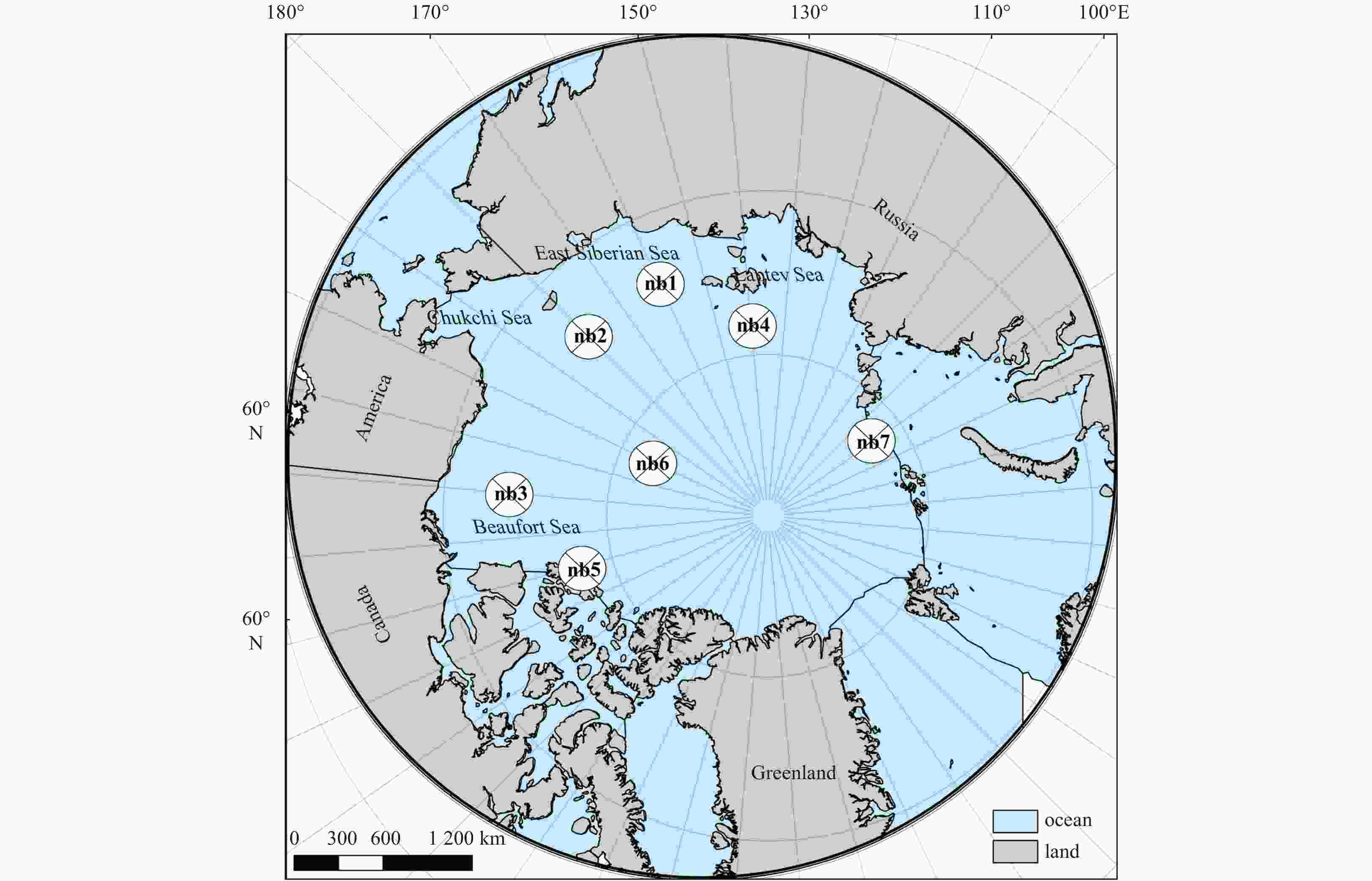
Figure 3. Spatial distribution of the region where velocity data for buoys in the Arctic Ocean are obtained. The buoys are numbered as nbx with x being 1 to 7.
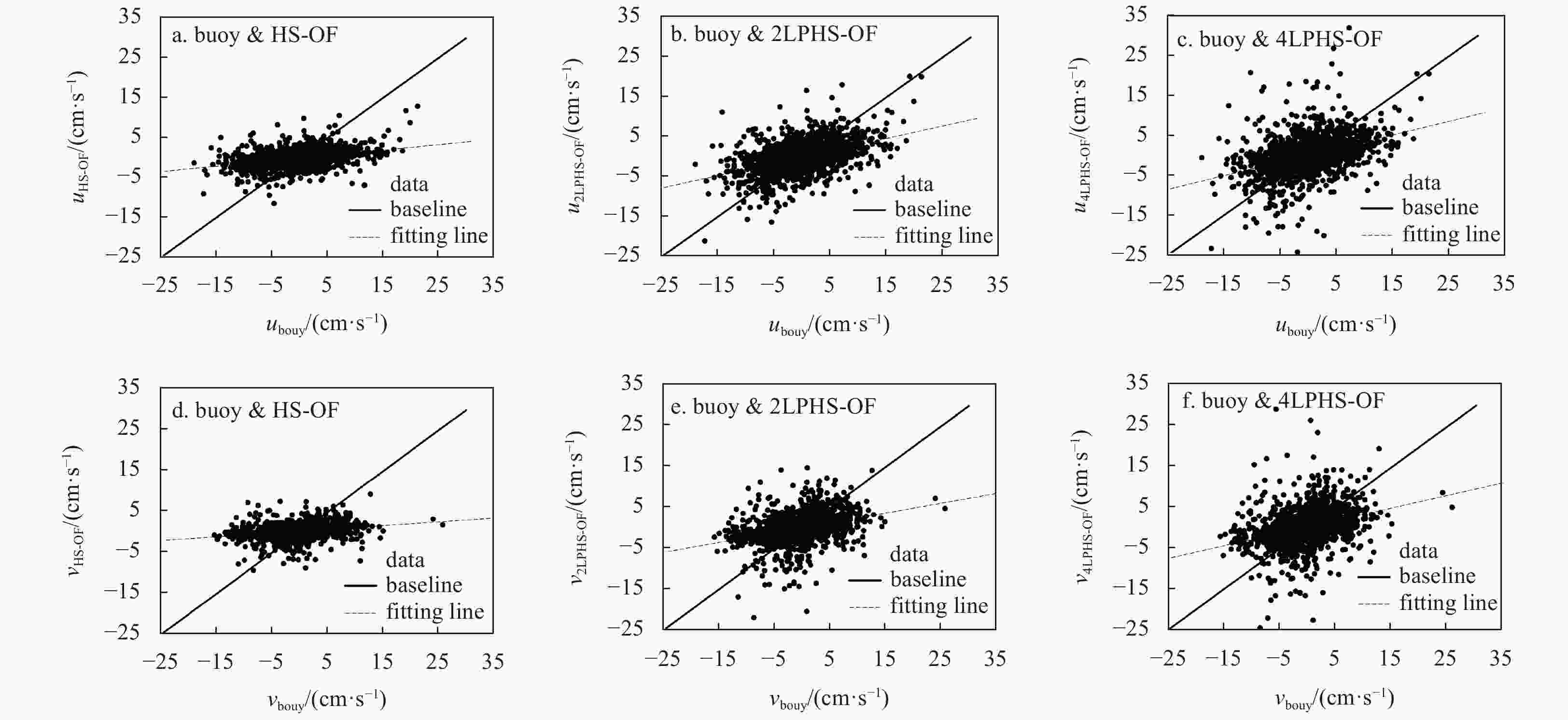
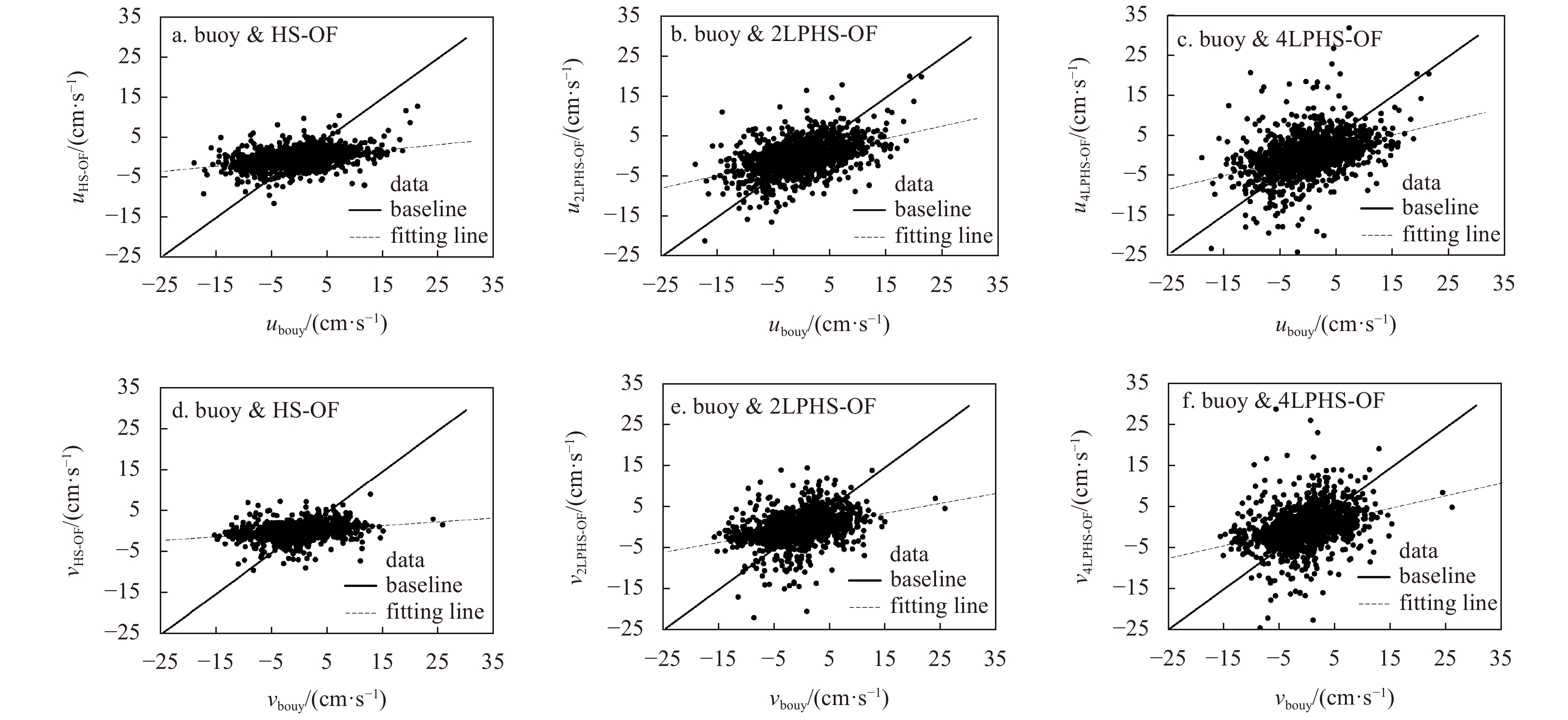
Figure 4. Scatterplots of the data obtained by the HS-OF, 2LPHS-OF and 4LPHS-OF methods versus the buoy data in the u (x) and v (y) directions. a, b and c. HS-OF velocity, 2LPHS-OF velocity and 4LPHS-OF velocity in the u-direction; and d, e and f. HS-OF velocity, 2LPHS-OF velocity and 4LPHS-OF velocity in the v-direction.
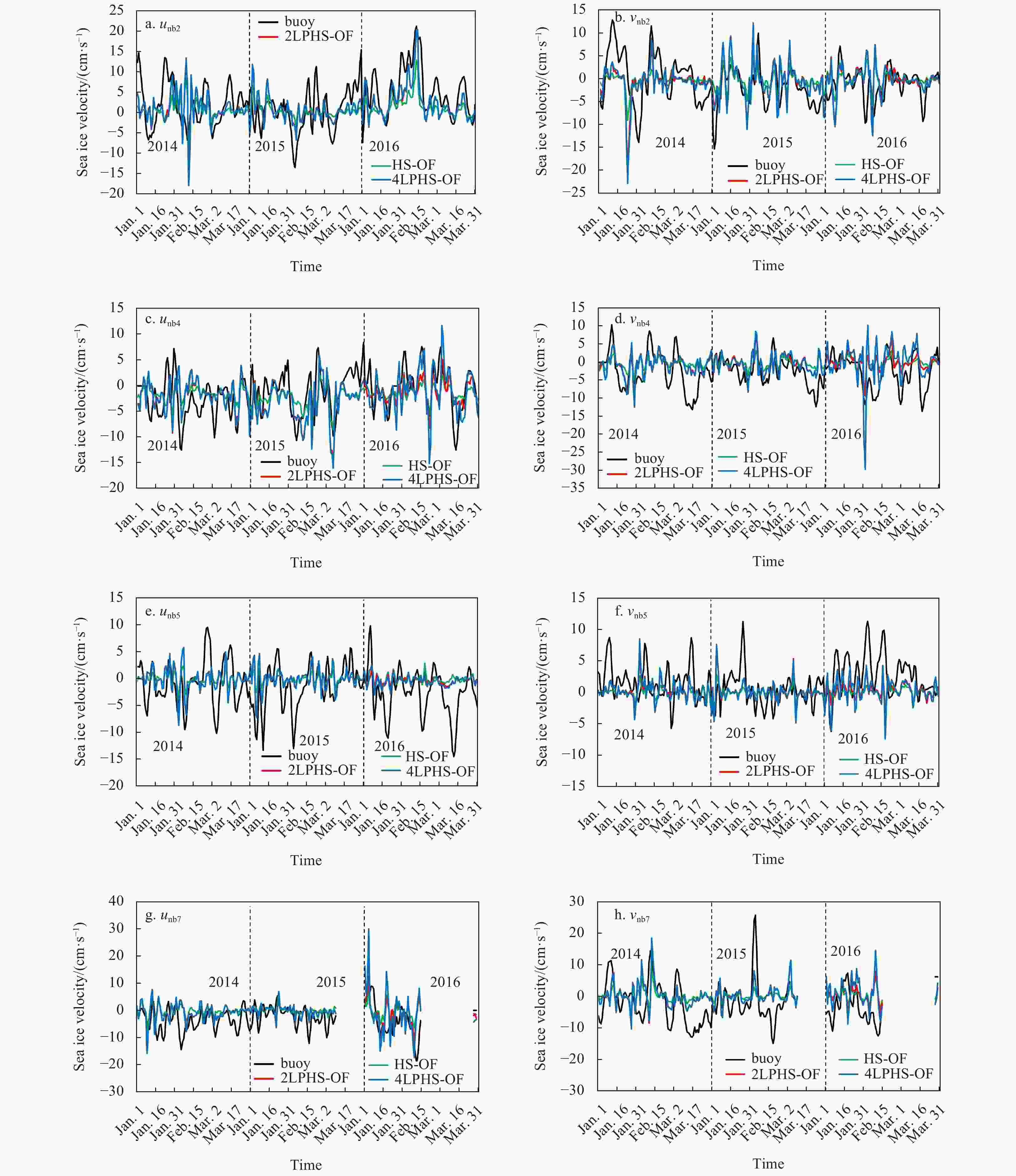
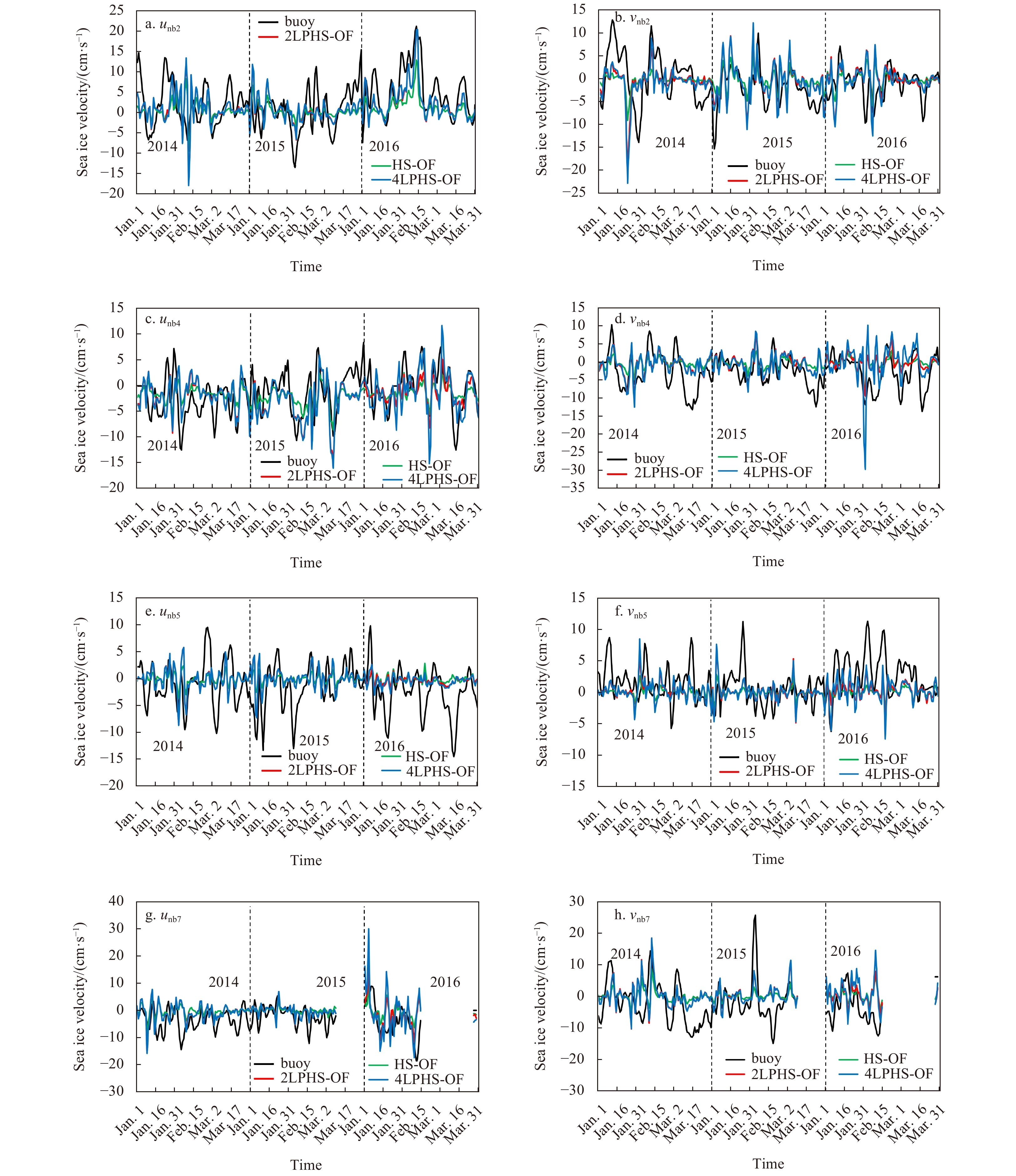
Figure 5. The daily sea ice velocity in winter from 2014 to 2016 in the u-direction and v-direction, which are obtained from buoys and by the HS-OF, 2LPHS-OF and 4LPHS-OF methods. a, c, e and g. Velocities at the nb2, nb4, nb5 and nb7 positions in the u-direction; and b, d, f and h. velocity at the nb2, nb4, nb5 and nb7 positions in the v-direction.

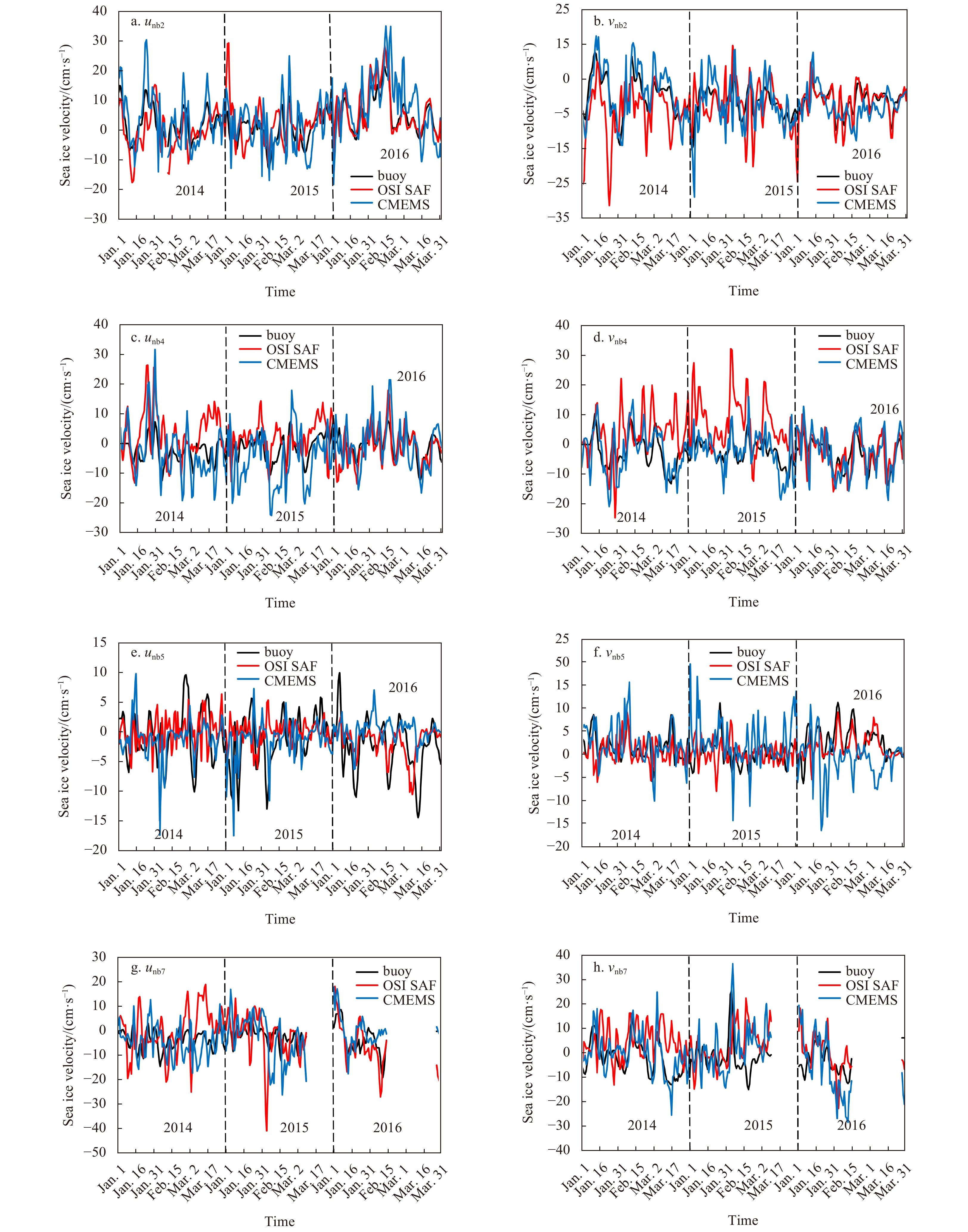
Figure 6. The daily sea ice velocity in winter from 2014 to 2016 in the u-direction and v-direction, which are obtained from buoys and the OSI SAF and CMEMS dataset. a, c, e and g. Velocities at the nb2, nb4, nb5 and nb7 positions in the u-direction; and b, d, f and h. velocities at the nb2, nb4, nb5 and nb7 positions in the v-direction.

Figure 7. Spatial distribution of the sea ice drift velocity on the 1st and 15th days of each month in the Arctic in 2016. The blue box indicates the occurrence of the Arctic cyclone, and the black box indicates the occurrence of the Arctic anticyclone, including the Beaufort Gyre.
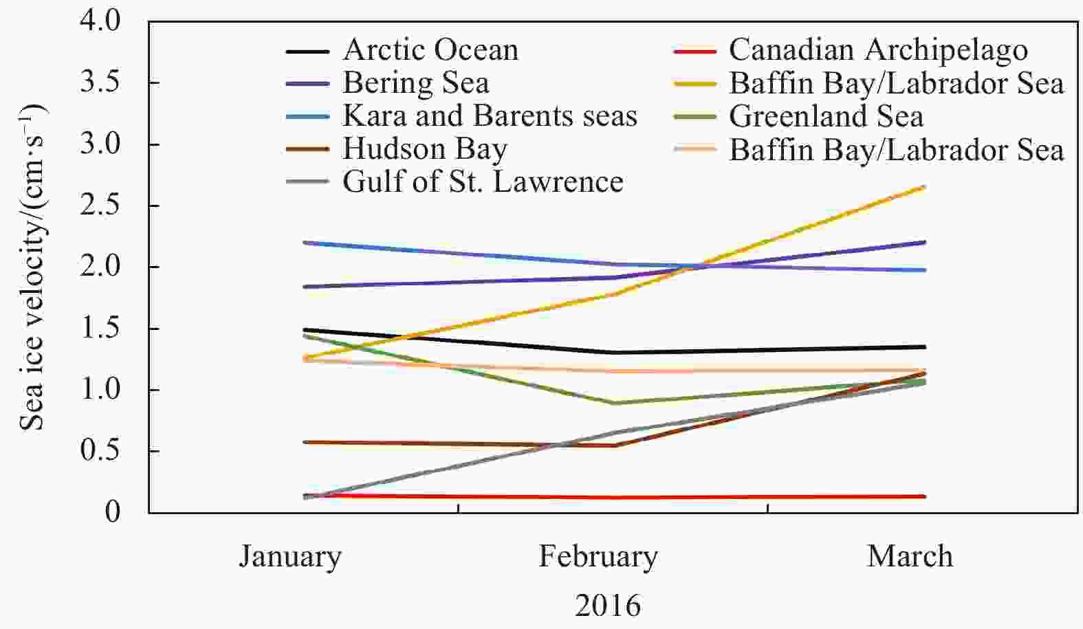
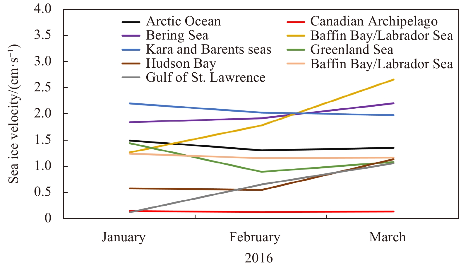
Figure 8. The monthly sea ice velocity in nine subregions from January to March, 2016.
Table 1. Statistics for three sea ice drift datasets
Data provider NSIDC OSI SAF CMEMS Sensor AMSR-E, AVHRR, drifting buoys,
SMMR, SSM/I, SSMISAMSR-2, SSMIS, ASCAT AMSR-E, AMSR-2, SSM/I, SSMIS,
QuickSCAT, ASCATSpatial resolution 25 km×25 km 62.5 km×62.5 km 12.5 km×12.5 km Method MCC CMCC CMCC, model  下载: 导出CSV
Table 2. Accuracy evaluation of the HS-OF, 2LPHS-OF and 4LPHS-OF methods for the buoy velocity positions (in the u-direction and v-direction) through RMSE, ME, MAE, and P from 2014 to 2016 (winter)
unb1 vnb1 HS-OF 2LPHS-OF 4LPHS-OF HS-OF 2LPHS-OF 4LPHS-OF RMSE/(cm·s–1) 4.83 4.79 4.88 4.20 3.99 3.96 ME/(cm·s–1) –1.12 –0.79 –0.76 1.60 1.37 1.26 MAE/(cm·s–1) 3.63 3.63 3.72 3.10 2.97 2.91 P 0.44 0.62 0.58 0.58 0.70 0.71 unb2 vnb2 HS-OF 2LPHS-OF 4LPHS-OF HS-OF 2LPHS-OF 4LPHS-OF RMSE/(cm·s–1) 5.57 5.11 5.18 4.46 4.65 4.71 ME/(cm·s–1) –1.95 –1.19 –1.17 0.74 0.47 0.35 MAE/(cm·s–1) 4.40 3.98 4.00 3.35 3.46 3.43 P 0.79 0.84 0.83 0.52 0.66 0.68 unb3 vnb3 HS-OF 2LPHS-OF 4LPHS-OF HS-OF 2LPHS-OF 4LPHS-OF RMSE/(cm·s–1) 5.06 4.23 4.28 3.84 4.67 5.34 ME/(cm·s–1) –0.49 –0.29 -0.31 –1.78 –1.04 –0.99 MAE/(cm·s–1) 4.01 3.31 3.33 3.04 3.50 3.91 P 0.89 0.93 0.92 0.67 0.73 0.69 unb4 vnb4 HS-OF 2LPHS-OF 4LPHS-OF HS-OF 2LPHS-OF 4LPHS-OF RMSE/(cm·s–1) 3.86 4.08 4.27 4.90 4.53 5.14 ME/(cm·s–1) –0.29 –0.62 –0.59 2.24 1.92 2.03 MAE/(cm·s–1) 3.06 3.20 3.32 3.80 3.47 3.84 P 0.64 0.69 0.72 0.64 0.76 0.62 unb5 vnb5 HS-OF 2LPHS-OF 4LPHS-OF HS-OF 2LPHS-OF 4LPHS-OF RMSE/(cm·s–1) 4.48 4.40 4.37 3.39 3.39 3.48 ME/(cm·s–1) 1.57 1.47 1.44 –1.48 –1.36 –1.33 MAE/(cm·s–1) 3.37 3.30 3.27 2.53 2.58 2.62 P 0.34 0.48 0.50 0.30 0.42 0.39 unb6 vnb6 HS-OF 2LPHS-OF 4LPHS-OF HS-OF 2LPHS-OF 4LPHS-OF RMSE/(cm·s–1) 4.92 5.25 8.12 4.20 4.67 6.80 ME/(cm·s–1) 1.41 1.14 1.16 0.61 0.44 0.76 MAE/(cm·s–1) 3.69 3.92 5.80 3.34 3.59 4.49 P 0.35 0.44 0.36 0.43 0.52 0.61 unb7 vnb7 HS-OF 2LPHS-OF 4LPHS-OF HS-OF 2LPHS-OF 4LPHS-OF RMSE/(cm·s–1) 4.72 4.70 5.30 5.92 5.99 6.17 ME/(cm·s–1) 2.86 2.37 2.37 2.30 2.42 2.54 MAE/(cm·s–1) 4.13 4.04 4.45 5.36 5.42 5.55 P 0.38 0.54 0.52 0.25 0.37 0.33
下载: 导出CSV
Table 3. Overall accuracy evaluation of the HS-OF, 2LPHS-OF and 4LPHS-OF methods in the u-direction and v-direction through the RMSE, ME, MAE, and P based on buoy velocity from 2014 to 2016 (winter, a total of 1 829 matchup data)
u v HS-OF 2LPHS-OF 4LPHS-OF HS-OF 2LPHS-OF 4LPHS-OF RMSE/(cm·s–1) 4.89 4.76 5.45 4.56 4.70 5.29 ME/(cm·s–1) 0.19 0.22 0.23 0.54 0.54 0.59 MAE/(cm·s–1) 3.74 3.61 3.97 3.44 3.48 3.76 P 0.61 0.70 0.65 0.50 0.60 0.59 Note: The bolded values are the 2LPHS-OF volocity.
下载: 导出CSV
Table 4. Accuracy evaluation of the OSI SAF and CMEMS vectors in the u- and v-directions through the RMSE, ME, MAE, and P values based on buoy velocity
u v OSI SAF CMEMS OSI SAF CMEMS RMSE/(cm·s–1) 6.28 (24%) 6.36 (25%) 6.98 (33%) 5.60 (16%) ME/(cm·s–1) 0.57 (60%) 0.15 (–56%) 1.22 (56%) 0.35 (–55%) MAE/(cm·s–1) 4.50 (20%) 4.93 (27%) 4.73 (26%) 4.16 (16%) P 0.64 (8%) 0.87 (–25%) 0.43 (41%) 0.78 (–29%) Note: The values in brackets indicate the percentage improvement of the accuracy indices of the 2LPHS-OF velocity relative to the accuracy indices of the other data.
下载: 导出CSV
Table 5. Evaluation of the 2LPHS-OF vectors in the u- and v-directions through the RMSE, ME, MAE, and P based on NSIDC velocity data from 2014 to 2016
RMSE/(cm·s−1) ME/(cm·s−1) MAE/(cm·s−1) P u 1.90 0.90 1.45 0.62 v 1.99 0.91 1.64 0.80
下载: 导出CSV
Table 6. Statistics for sea ice velocity in nine subregions of the Arctic
Region Mean
/(cm·s−1)SD
/(cm·s−1)Speed rate
/(cm·s−1·d−1)Arctic Ocean 1.39 0.70 –0.0030 Canadian Archipelago 0.14 0.08 –0.0002 Bering Sea 1.20 1.26 0.0050 Seas of Okhotsk and Japan 1.91 1.26 0.02501) Kara and Barents seas 2.07 1.10 –0.0060 Greenland Sea 1.15 0.74 –0.0030 Hudson Bay 0.77 0.92 0.00902) Baffin Bay/Labrador Sea 1.20 0.56 –0.0010 Gulf of St. Lawrence 0.62 1.00 0.0150 Note: 1) Probability value < 0.01. 2) Probability value < 0.05. Bolded values indicate a speed rate greater than 0.
下载: 导出CSV
-
[1] Agnew T A, Le Hao, Hirose T. 1997. Estimation of large-scale sea-ice motion from SSM/I 85.5 GHz imagery. Annals of Glaciology, 25: 305–311. doi: 10.3189/S0260305500014191 [2] Allison I. 1989. Pack-ice drift off East Antarctica and some implications. Annals of Glaciology, 12: 1–8. doi: 10.3189/S0260305500006881 [3] Arrigo K R, Van Dijken G L. 2011. Secular trends in Arctic Ocean net primary production. Journal of Geophysical Research: Oceans, 116(C9): C09011 [4] Berg A, Eriksson L E B. 2014. Investigation of a hybrid algorithm for sea ice drift measurements using synthetic aperture radar images. IEEE Transactions on Geoscience and Remote Sensing, 52(8): 5023–5033. doi: 10.1109/TGRS.2013.2286500 [5] Borcea L, Callaghan T, Papanicolaou G. 2012. Synthetic aperture radar imaging and motion estimation via robust principal component analysis. SIAM Journal on Imaging Sciences, 6(3): 1445–1476 [6] Cavalieri D J, Parkinson C L, Vinnikov K Y. 2003. 30-year satellite record reveals contrasting Arctic and Antarctic decadal sea ice variability. Geophysical Research Letters, 30(18): 1970 [7] Choudhary B K, Sinha N K, Shanker P. 2012. Pyramid method in image processing. Journal of Information Systems and Communication, 3(1): 269–273 [8] Copernicus Marine Service (CMEMS). 2020. Product user manual for Arctic Ocean physical and BGC analysis and forecasting products. Issue 5.12. http://marine.copernicus.eu/documents/PUM/CMEMS-ARC-PUM-002-ALL.pdf [2020-04/2021-01-10] [9] Comiso J C, Meier W N, Gersten R. 2017. Variability and trends in the arctic sea ice cover: results from different techniques. Journal of Geophysical Research:Oceans, 122(8): 6883–6900. doi: 10.1002/2017JC012768 [10] Deng Juan. 2014. Northern Hemisphere sea ice variability and its relationship with climate factors (in Chinese) [dissertation]. Nanjing: Nanjing University [11] Emery W J, Fowler C W, Maslanik J A. 1997. Satellite-derived maps of Arctic and Antarctic sea ice motion: 1988 to 1994. Geophysical Research Letters, 24(8): 897–900. doi: 10.1029/97GL00755 [12] Fleet D, Weiss Y. 2006. Optical flow estimation. In: Paragios N, Chen Yunmei, Faugeras O, eds. Handbook of Mathematical Models in Computer Vision. Boston: Springer, 237–257 [13] Girard-Ardhuin F, Ezraty R. 2012. Enhanced arctic sea ice drift estimation merging radiometer and scatterometer data. IEEE Transactions on Geoscience and Remote Sensing, 50(7): 2639–2648. doi: 10.1109/TGRS.2012.2184124 [14] Gutiérrez S, Long D G. 2003. Optical flow and scale-space theory applied to sea-ice motion estimation in Antarctica. In: Proceedings of 2003 IEEE International Geoscience and Remote Sensing Symposium. Toulouse: IEEE, 2805–2807 [15] Horn B K P, Schunck B G. 1981. Determining optical flow. Artificial Intelligence, 17(1−3): 185–203. doi: 10.1016/0004-3702(81)90024-2 [16] Ke Ruimin, Li Zhibin, Tang Jinjun, et al. 2019. Real-time traffic flow parameter estimation from UAV video based on ensemble classifier and optical flow. IEEE Transactions on Intelligent Transportation Systems, 20(1): 54–64. doi: 10.1109/TITS.2018.2797697 [17] Ke Changqing, Peng Haitao, Sun Bo, et al. 2013. Spatio-temporal variability of Arctic sea ice from 2002 to 2011. Journal of Remote Sensing (in Chinese), 17(2): 452–466 [18] Komarov A S, Barber D G. 2014. Sea ice motion tracking from sequential dual-polarization Radarsat-2 Images. IEEE Transactions on Geoscience and Remote Sensing, 52(1): 121–136. doi: 10.1109/TGRS.2012.2236845 [19] Kwok R, Schweiger A, Rothrock D A, et al. 1998. Sea ice motion from satellite passive microwave imagery assessed with ERS SAR and buoy motions. Journal of Geophysical Research:Oceans, 103(C4): 8191–8214. doi: 10.1029/97JC03334 [20] Kwok R, Spreen G, Pang S. 2013. Arctic sea ice circulation and drift speed: decadal trends and ocean currents. Journal of Geophysical Research: Oceans, 118(5): 2408–2425. doi: 10.1002/jgrc.20191 [21] Lan Jinhui, Li Jian, Hu Guangda, et al. 2014. Vehicle speed measurement based on gray constraint optical flow algorithm. Optik, 125(1): 289–295. doi: 10.1016/j.ijleo.2013.06.036 [22] Lavergne T, Eastwood S, Teffah Z, et al. 2010. Sea ice motion from low-resolution satellite sensors: an alternative method and its validation in the arctic. Journal of Geophysical Research: Oceans, 115(C10): C10032 [23] Lehtiranta J, Siiriä S, Karvonen J. 2015. Comparing C- and L-Band SAR images for sea ice motion estimation. The Cryosphere, 9(1): 357–366. doi: 10.5194/tc-9-357-2015 [24] Li Haili, Ke Changqing. 2017. Open water variability in the North Pole from 1982 to 2016. Haiyang Xuebao (in Chinese), 39(12): 109–121 [25] Li Haili, Ke Changqing, Zhu Qinghui, et al. 2019. Spatial-temporal variations in net primary productivity in the Arctic from 2003 to 2016. Acta Oceanologica Sinica, 38(8): 111–121. doi: 10.1007/s13131-018-1274-5 [26] Lim A, Ramesh B, Yang Yue, et al. 2019. Real-time optical flow-based video stabilization for unmanned aerial vehicles. Journal of Real-Time Image Processing, 16(6): 1975–1985. doi: 10.1007/s11554-017-0699-y [27] Liu A K, Cavalieri D J. 1998. On sea ice drift from the wavelet analysis of the defense meteorological satellite program (DMSP) special sensor microwave imager (SSM/I) data. International Journal of Remote Sensing, 19(7): 1415–1423. doi: 10.1080/014311698215522 [28] Liu Yige, Ke Changqing, Zhang Jie. 2019. Analysis of kinematic characteristics of Antarctic sea ice from 1979 to 2014. Chinese High Technology Letters (in Chinese), 29(1): 90–98 [29] Liu A K, Zhao Yunhe, Wu S Y. 1999. Arctic sea ice drift from wavelet analysis of NSCAT and special sensor microwave imager data. Journal of Geophysical Research: Oceans, 104(C5): 11529–11538. doi: 10.1029/1998JC900115 [30] Mäkynen M, Haapala J, Aulicino G, et al. 2020. Satellite observations for detecting and forecasting sea-ice conditions: a summary of advances made in the SPICES project by the EU’s Horizon 2020 Programme. Remote Sensing, 12(7): 1214. doi: 10.3390/rs12071214 [31] Massom R A, Stammerjohn S E. 2010. Antarctic sea ice change and variability—physical and ecological implications. Polar Science, 4(2): 149–186. doi: 10.1016/j.polar.2010.05.001 [32] Meier W N, Dai Mingrui. 2006. High-resolution sea-ice motions from AMSR-E imagery. Annals of Glaciology, 44: 352–356. doi: 10.3189/172756406781811286 [33] Min Chao, Mu Longjiang, Yang Qinghua, et al. 2019. Sea ice export through the Fram Strait derived from a combined model and satellite data set. The Cryosphere, 13(12): 3209–3224. doi: 10.5194/tc-13-3209-2019 [34] Muckenhuber S, Korosov A A, Sandven S. 2016. Open-source feature-tracking algorithm for sea ice drift retrieval from sentinel-1 SAR imagery. The Cryosphere, 10(2): 913–925. doi: 10.5194/tc-10-913-2016 [35] Muckenhuber S, Sandven S. 2018. Sea ice drift data for Fram Strait derived from a feature-tracking algorithm applied on sentinel-1 SAR imagery. Data in Brief, 18(2018): 1410–1415. doi: 10.1016/j.dib.2018.04.034 [36] Ninnis R M, Emery W J, Collins M J. 1986. Automated extraction of pack ice motion from advanced very high resolution radiometer imagery. Journal of Geophysical Research:Oceans, 91(C9): 10725–10734. doi: 10.1029/JC091iC09p10725 [37] NSIDC. 2019. Polar pathfinder daily 25 km EASE-grid sea ice motion vectors, version 4-user guide. https://nsidc.org/data/NSIDC-0116/versions/4 [2019-02-25/2020-01-08] [38] Cavalieri D J, Parkinson C L. 2012. Arctic sea ice variability and trends, 1979–2010. The Cryosphere, 6(4): 881–889 [39] Parkinson C L, Cavalieri D J, Gloersen P, et al. 1999. Arctic sea ice extents, areas, and trends, 1978–1996. Journal of Geophysical Research: Oceans, 104(C9): 20837–20856. doi: 10.1029/1999JC900082 [40] Peng Ge, Meier W N. 2018. Temporal and regional variability of arctic sea-ice coverage from satellite data. Annals of Glaciology, 59(76pt2): 191–200. doi: 10.1017/aog.2017.32 [41] Petrou Z I, Tian Yingli. 2017. High-resolution sea ice motion estimation with optical flow using satellite spectroradiometer data. IEEE Transactions on Geoscience and Remote Sensing, 55(3): 1339–1350. doi: 10.1109/TGRS.2016.2622714 [42] Petrou Z I, Xian Yang, Tian Yingli. 2018. Towards breaking the spatial resolution barriers: an optical flow and super-resolution approach for sea ice motion estimation. ISPRS Journal of Photogrammetry and Remote Sensing, 138: 164–175. doi: 10.1016/j.isprsjprs.2018.01.020 [43] Petty A A, Webster M, Boisvert L, et al. 2018. The NASA Eulerian snow on sea ice model (NESOSIM) v1.0: initial model development and analysis. Geoscientific Model Development, 11(11): 4577–4602. doi: 10.5194/gmd-11-4577-2018 [44] Qiu Bowei, Li Chunhua, Guan Changlong, et al. 2019. The influence of sea ice drift on the distribution of multiyear ice. Transactions of Oceanology and Limnology (in Chinese), (3): 1–11 [45] Rossel R A V, Webster R. 2012. Predicting soil properties from the australian soil visible-near infrared spectroscopic database. European Journal of Soil Science, 63(6): 848–860. doi: 10.1111/j.1365-2389.2012.01495.x [46] Rostosky P, Spreen G, Farrell S L, et al. 2018. Snow depth retrieval on Arctic sea ice from passive microwave radiometers—improvements and extensions to multiyear ice using lower frequencies. Journal of Geophysical Research: Oceans, 123(10): 7120–7138. doi: 10.1029/2018JC014028 [47] Sakov P, Counillon F, Bertino L, et al. 2012. TOPAZ4: an ocean-sea ice data assimilation system for the North Atlantic and Arctic. Ocean Science, 8(4): 633–656. doi: 10.5194/os-8-633-2012 [48] Tian Zhongxiang, Li Chunhua, Zhang Lin, et al. 2012. Climatology characteristics of Arctic sea ice motion. Marine Forecasts (in Chinese), 29(6): 66–73 [49] Wang Liya, He Yijun, Zhang Biao, et al. 2017. Retrieval of Arctic sea ice drift using HY-2 satellite scanning microwave radiometer data. Haiyang Xuebao (in Chinese), 39(9): 110–120 [50] Wu Qing, Lang Wenhui, Zhang Xi, et al. 2014. Sea ice drift tracking in the Bohai Sea based on optical flow. In: Proceedings of SPIE 9159 Sixth International Conference on Digital Image Processing (ICDIP 2014). Athens: SPIE [51] Zhang Jinlun, Rothrock D, Steele M. 2000. Recent changes in Arctic sea ice: the interplay between ice dynamics and thermodynamics. Journal of Climate, 13(17): 3099–3114. doi: 10.1175/1520-0442(2000)013<3099:RCIASI>2.0.CO;2 [52] Zhao Yunhe, Liu A K. 2007. Arctic sea-ice motion and its relation to pressure field. Journal of Oceanography, 63(3): 505–515. doi: 10.1007/s10872-007-0045-2 [53] Zhu Wenbin, Jia Shaofeng, Lv Aifeng. 2014. Monitoring the fluctuation of Lake Qinghai using multi-source remote sensing data. Remote Sensing, 6(11): 10457–10482. doi: 10.3390/rs61110457 [54] Zuo Zhengdao, Gao Guoping, Cheng Lingqiao, et al. 2016. Preliminary analysis of kinematic characteristics of Arctic sea ice from 1979 to 2012. Haiyang Xuebao (in Chinese), 38(5): 57–69 -


 点击查看大图

计量
- 文章访问数: 632
- HTML全文浏览量: 224
- PDF下载量: 34
- 被引次数: 0