

A multi-scale high-order recursive filter approach for the sea ice concentration analysis
-
Abstract: With the development and deployment of observation systems in the ocean, more precise passive and active microwave data are becoming available for the weather forecasting and the climate monitoring. Due to the complicated variability of the sea ice concentration (SIC) in the marginal ice zone and the scarcity of high-precision sea ice data, how to use less data to accurately reconstruct the sea ice field has become an urgent problem to be solved. A reconstruction method for gridding observations using the variational optimization technique, called the multi-scale high-order recursive filter (MHRF), which is a combination of Van Vliet fourth-order recursive filter and the three-dimensional variational (3D-VAR) analysis, has been designed in this study to reproduce the refined structure of sea ice field. Compared with the existing spatial multi-scale first-order recursive filter (SMRF) in which left and right filter iterative processes are executed many times, the MHRF scheme only executes the same filter process once to reduce the analysis errors caused by multiple filters and improve the filter precision. Furthermore, the series connected transfer function in the high-order recursive filter is equivalently replaced by the paralleled one, which can carry out the independent filter process in every direction in order to improve the filter efficiency. Experimental results demonstrate that this method possesses a good potential in extracting the observation information to successfully reconstruct the SIC field in computational efficiency.
-
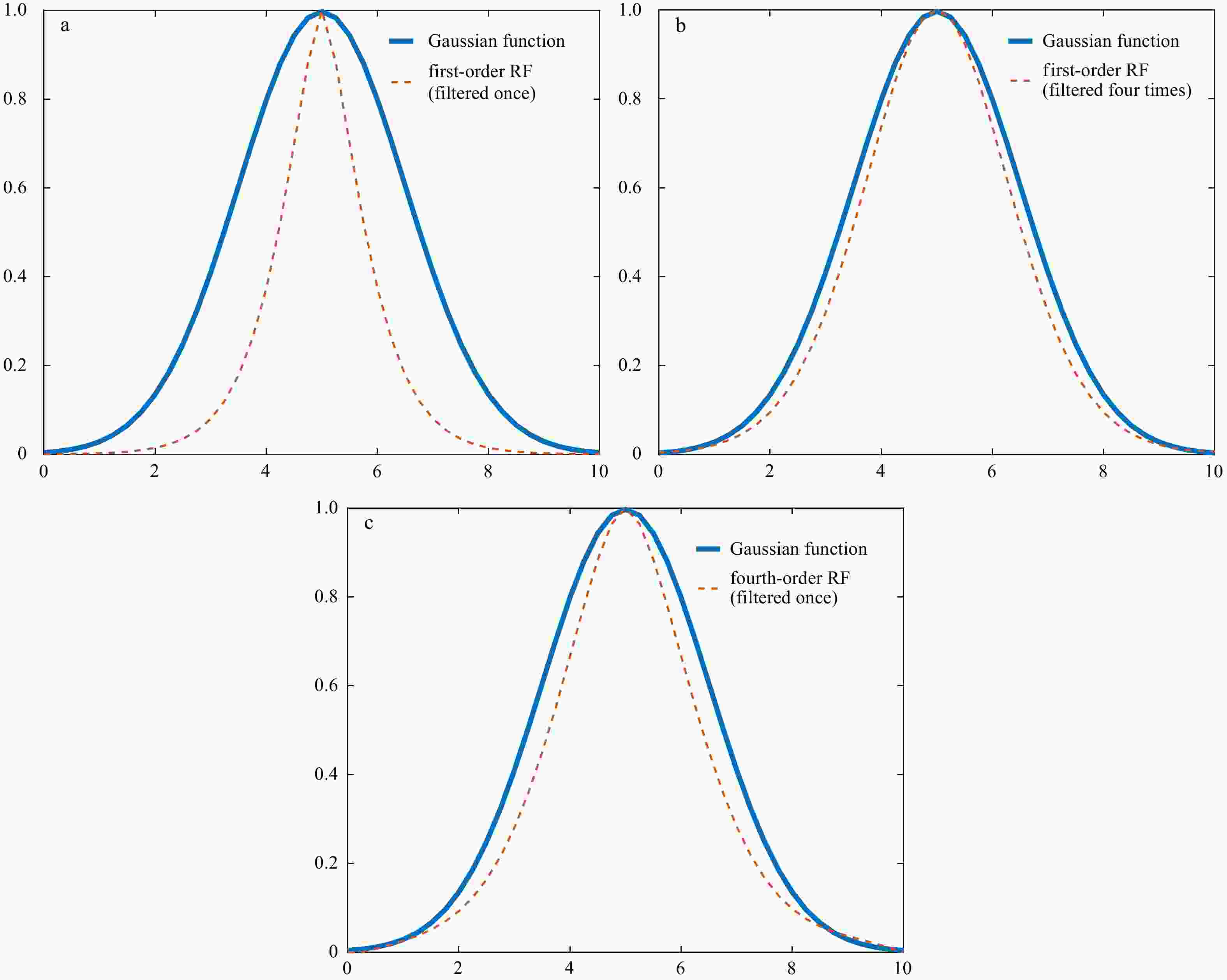
Figure 2. Comparison of one-dimensional recursive filter results (dotted line) with the Gaussian function (solid line): the first-order recursive filter once (a); the first-order recursive filter four times (b); Van Vliet fourth-order recursive filter once (c).

Figure 3. The spread of observational information using the L-BFGS scheme when
$ \beta $ = 1 (a), 2 (b), 4 (c) and 6 (d), respectively.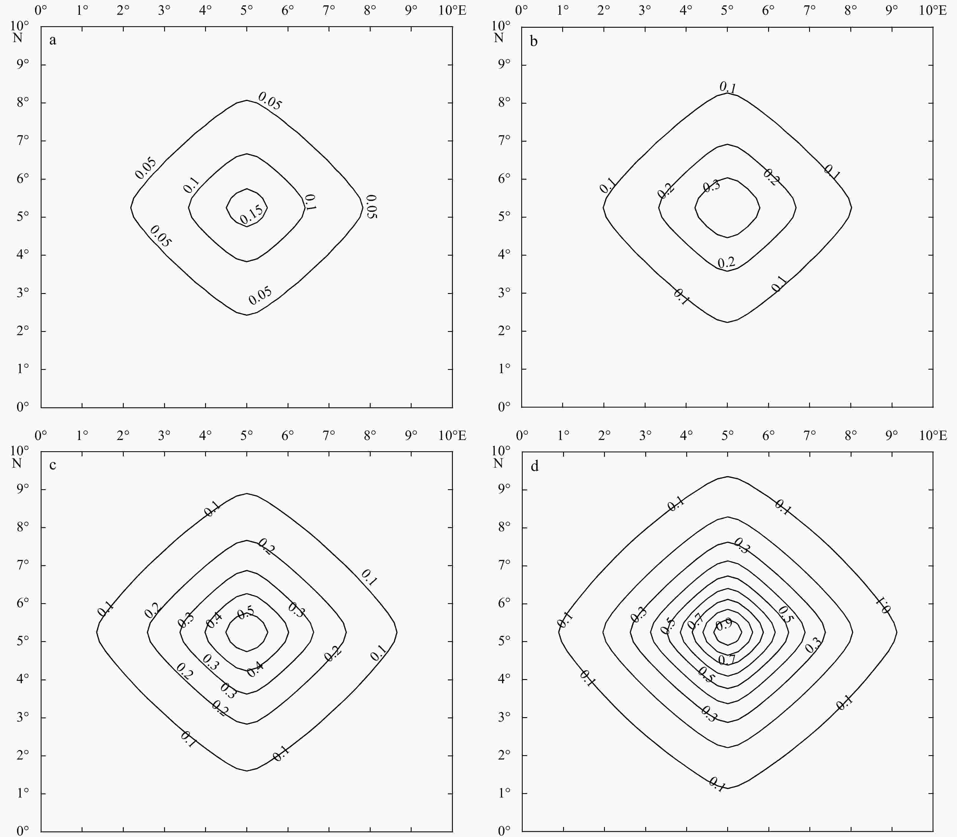
Figure 4. The spread of observational information in the multi-scale high-order recursive filter scheme when
$ \theta $ = 0.97. a–d are the results at iteration 2, 5, 8 and 24, respectively.
Figure 5. The true SIC field of the Arctic Ocean constructed based on the SSMIS SIC on August 10, 2020 (a), and the locations of “observations” (b).

Figure 6. Analyzed field solved by using the L-BFGS scheme when
$ \beta $ =4 (a), 10 (b), 15 (c) and 25 (d).
Figure 7. Analyzed field (left column) and the descent direction (
$-\nabla {J}$ ) (right column) solved using the L-BFGS scheme ($ \beta $ =4) at iteration 2 (a, b), 4 (c, d) and 8 (e, f), respectively.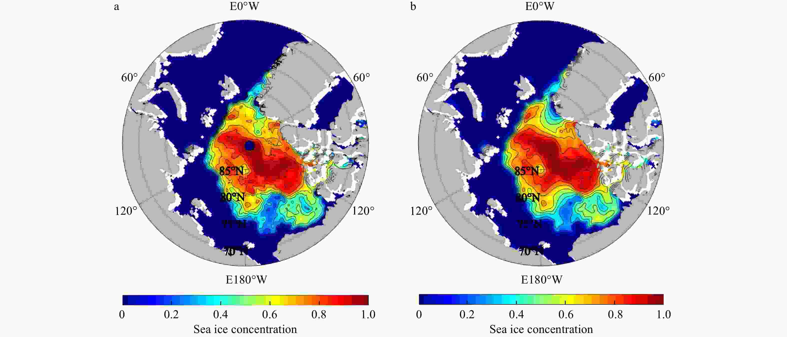
Figure 8. The true SIC (a) and the analysis result (b) from the MHRF scheme with
$ \beta= $ 0.99 and$ N= $ 125.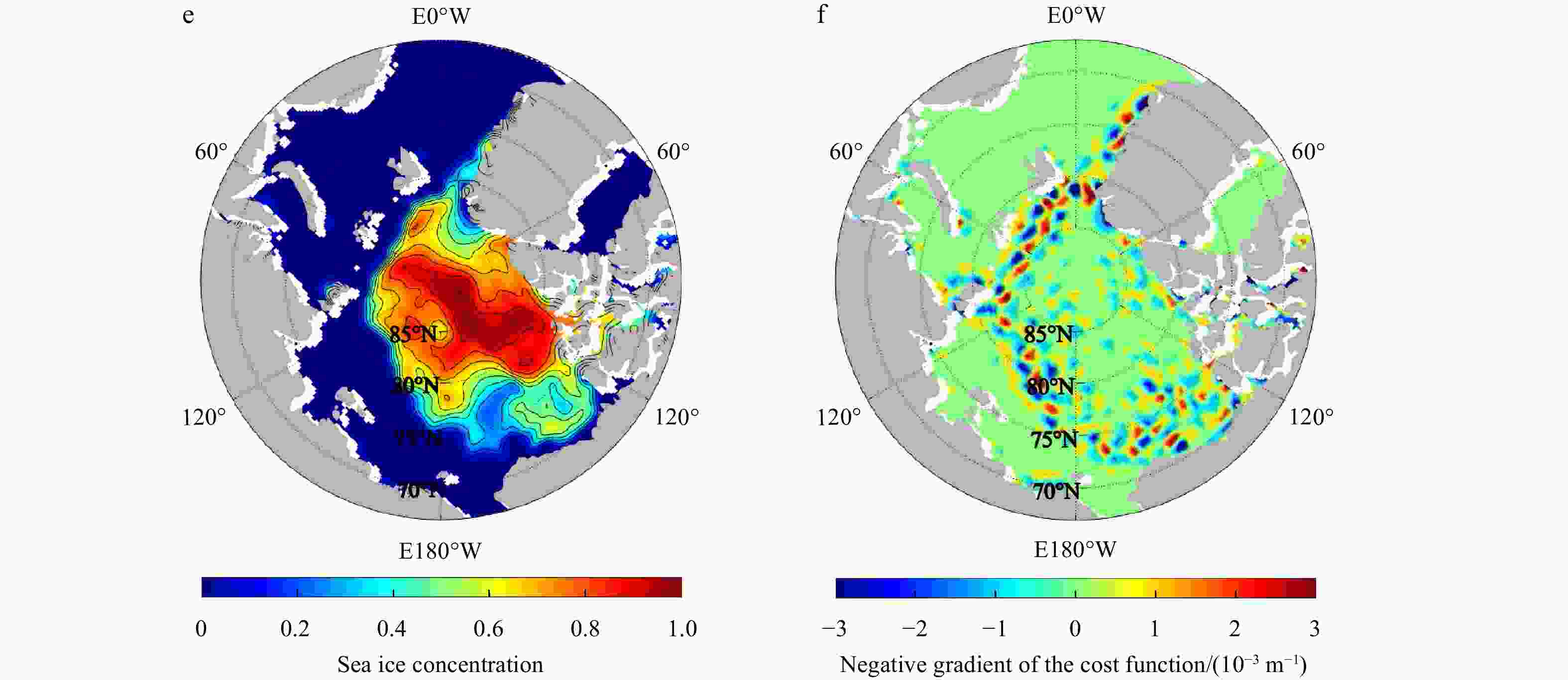
Figure 9. Analyzed field (left column) and the descent direction (right column) of the MHRF scheme (
$ \beta $ =0.99) at iteration 6 (a, b), 30 (c, d) and 55 (e, f).
Figure 11. The differences between the analyzed field and the true SIC field for the MHRF scheme (a) and the SMRF scheme (b).
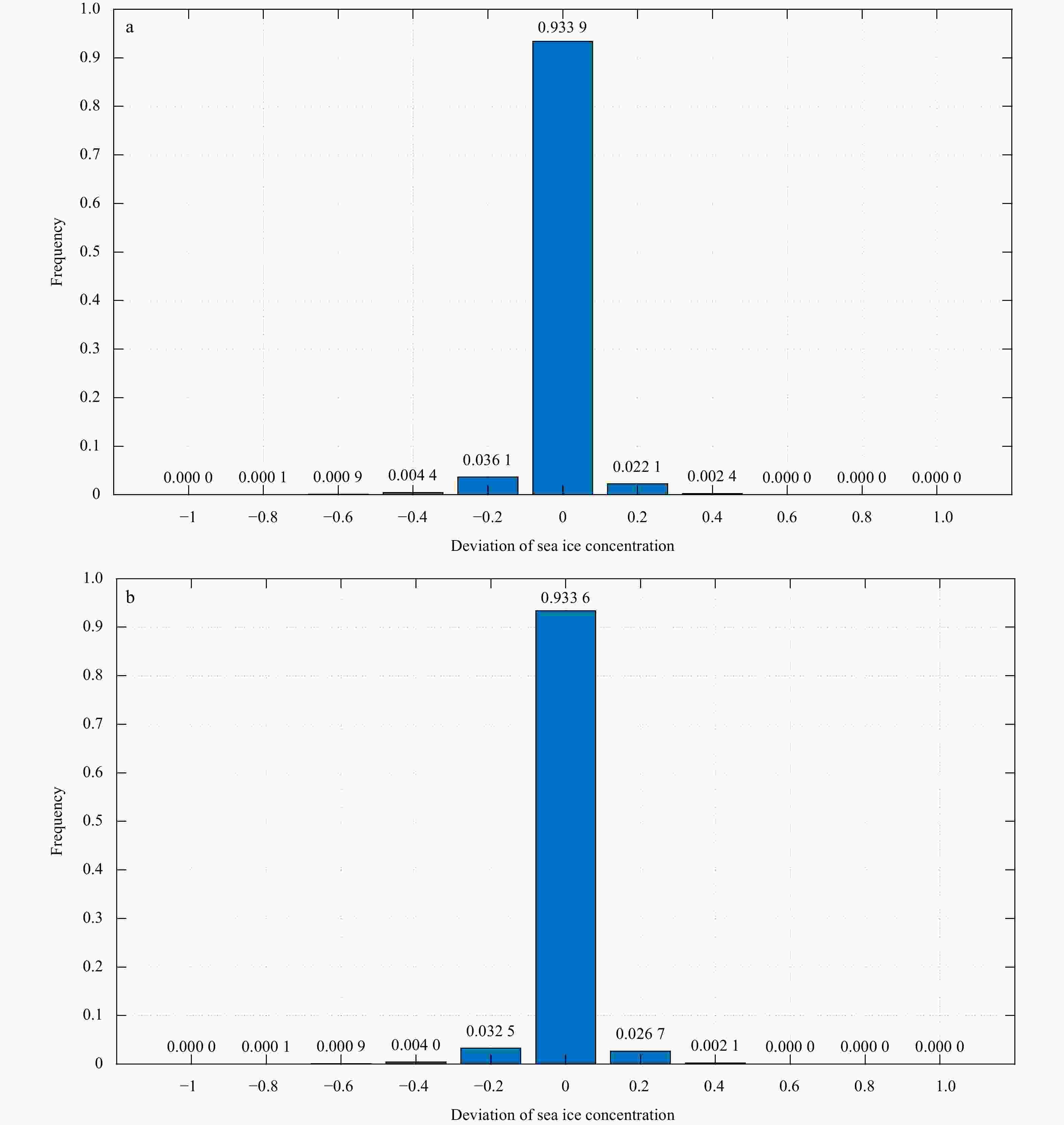
Figure 12. Histogram of the deviation between the analyzed field and the true SIC field for the MHRF scheme (a) and SMRF scheme (b).
Table 1. Comparison of RMSE and CPU computation time between the MHRF scheme and the SMRF scheme
RMSE The iteration steps CPU time/s MHRF scheme 0.059 8 125 3.303 SMRF scheme 0.058 7 500 23.438  下载: 导出CSV
-
[1] Cavalieri D J, Parkinson C L, DiGirolamo N, et al. 2012. Intersensor calibration between F13 SSMI and F17 SSMIS for global sea ice data records. IEEE Geoscience and Remote Sensing Letters, 9(2): 233–236. doi: 10.1109/LGRS.2011.2166754 [2] Derber J, Rosati A. 1989. A global oceanic data assimilation system. Journal of Physical Oceanography, 19(9): 1333–1347. doi: 10.1175/1520-0485(1989)019<1333:AGODAS>2.0.CO;2 [3] Gao Jidong, Xue Ming, Brewster K, et al. 2004. A three-dimensional variational data analysis method with recursive filter for Doppler radars. Journal of Atmospheric and Oceanic Technology, 21(3): 457–469. doi: 10.1175/1520-0426(2004)021<0457:ATVDAM>2.0.CO;2 [4] Hayden C M, Purser R J. 1995. Recursive filter objective analysis of meteorological fields: Applications to NESDIS operational processing. Journal of Applied Meteorology and Climatology, 34(1): 3–15. doi: 10.1175/1520-0450-34.1.3 [5] He Zhongjie, Xie Yuanfu, Li Wei, et al. 2008. Application of the sequential three-dimensional variational method to assimilating SST in a global ocean model. Journal of Atmospheric and Oceanic Technology, 25(6): 1018–1033. doi: 10.1175/2007jtecho540.1 [6] Huang Xiangyu. 2000. Variational analysis using spatial filters. Monthly Weather Review, 128(7): 2588–2600. doi: 10.1175/1520-0493(2000)128<2588:vausf>2.0.co;2 [7] Huang Bohua, Kinter J L, Schopf P S. 2002. Ocean data assimilation using intermittent analyses and continuous model error correction. Advances in Atmospheric Sciences, 19(6): 965–992. doi: 10.1007/s00376-002-0059-z [8] Li Dong, Wang Xidong, Zhang Xuefeng, et al. 2011. Multi-scale 3D-VAR based on diffusion filter. Marine Science Bulletin, 30(2): 164–171. doi: 10.3969/j.issn.1001-6392.2011.02.007 [9] Li Wei, Xie Yuanfu, He Zhongjie, et al. 2008. Application of the multigrid data assimilation scheme to the China Seas’ temperature forecast. Journal of Atmospheric and Oceanic Technology, 25(11): 2106–2116. doi: 10.1175/2008JTECHO510.1 [10] Lorenc A. 1992. Iterative analysis using covariance functions and filters. Quarterly Journal of the Royal Meteorological Society, 118(505): 569–591. doi: 10.1002/qj.49711850509 [11] Masina S, Pinardi N, Navarra A. 2001. A global ocean temperature and altimeter data assimilation system for studies of climate variability. Climate Dynamics, 17(9): 687–700. doi: 10.1007/s003820000142 [12] Maslanik J, Stroeve J C. 1999. Near-real-time DMSP SSMIS daily polar gridded sea ice concentrations. Boulder, CO, USA: National Snow and Ice Data Center [13] Moré J J, Thuente D J. 1994. Line search algorithms with guaranteed sufficient decrease. ACM Transactions on Mathematical Software, 20(3): 286–307. doi: 10.1145/192115.192132 [14] Purser R J, McQuigg R. 1982. A successive correction analysis scheme using recursive numerical filters. Bracknell, Berkshire, UK: National Meteorological Library [15] Purser R J, Wu Wanshu, Parrish D F, et al. 2003a. Numerical aspects of the application of recursive filters to variational statistical analysis. Part I: Spatially homogeneous and isotropic Gaussian covariances. Monthly Weather Review, 131(8): 1524–1535. doi: 10.1175//1520-0493(2003)131<1524:NAOTAO>2.0.CO;2 [16] Purser R J, Wu Wanshu, Parrish D F, et al. 2003b. Numerical aspects of the application of recursive filters to variational statistical analysis. Part II: Spatially inhomogeneous and anisotropic general covariances. Monthly Weather Review, 131(8): 1536–1548. doi: 10.1175//2543.1 [17] Van Vliet L J, Young I T, Verbeek P W. 1998. Recursive Gaussian derivative filters. In: Proceedings of the Fourteenth International Conference on Pattern Recognition. Brisbane, QLD, Australia: IEEE, 509–514 [18] Zeng Zhongyi. 2006. Inverse problems in atmospheric science. Taiwan: National Editorial Library, 306–307 [19] Zhang Xuefeng, Yang Lu, Fu Hongli, et al. 2020. A variational successive corrections approach for the sea ice concentration analysis. Acta Oceanologica Sinica, 39(9): 140–154. doi: 10.1007/s13131-020-1654-5 -


 点击查看大图

计量
- 文章访问数: 373
- HTML全文浏览量: 152
- PDF下载量: 19
- 被引次数: 0