

Epipelagic mesozooplankton communities in the northeastern Indian Ocean off Myanmar during the winter monsoon
-
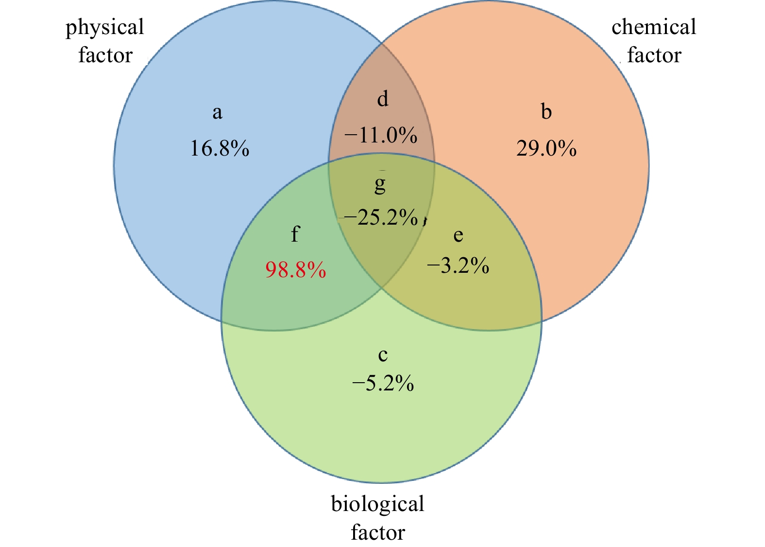
Abstract: The northern Andaman Sea off Myanmar is one of the relatively high productive regions in the Indian Ocean. The abundance, biomass and species composition of mesozooplankton and their relationships with environmental variables in the epipelagic zone (~200 m) were studied for the first time during the Sino-Myanmar joint cruise (February 2020). The mean abundance and biomass of mesozooplankton were (1916.7±1192.9) ind./m3 and (17.8±7.9) mg/m3, respectively. A total of 213 species (taxa) were identified from all samples. The omnivorous Cyclopoida Oncaea venusta and Oithona spp. were the top two dominant taxa. Three mesozooplankton communities were determined via cluster analysis: the open ocean in the Andaman Sea and the Bay of Bengal (Group A), the transition zone across the Preparis Channel (Group B), and nearshore water off the Ayeyarwady Delta and along the Tanintharyi Coast (Group C). Variation partitioning analysis revealed that the interaction of physical and biological factors explained 98.8% of mesozooplankton community spatial variation, and redundancy analysis revealed that column mean chlorophyll a concentration (CMCHLA) was the most important explanatory variable (43.1%). The abundance and biomass were significantly higher in Group C, the same as CMCHLA and column mean temperature (CMT) and in contrast to salinity, and CMT was the dominant factor. Significant taxon spatial variations were controlled by CMCHLA, salinity and temperature. This study suggested that mesozooplankton spatial variation was mainly regulated by physical processes through their effects on CMCHLA. The physical processes were simultaneously affected by heat loss differences, freshwater influx, eddies and depth.
-
Key words:
- mesozooplankton /
- Myanmar /
- epipelagic zone /
- physical processes /
- water column mean chlorophyll a
-
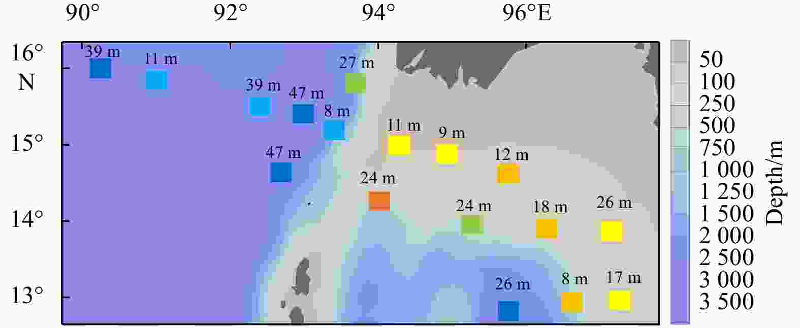
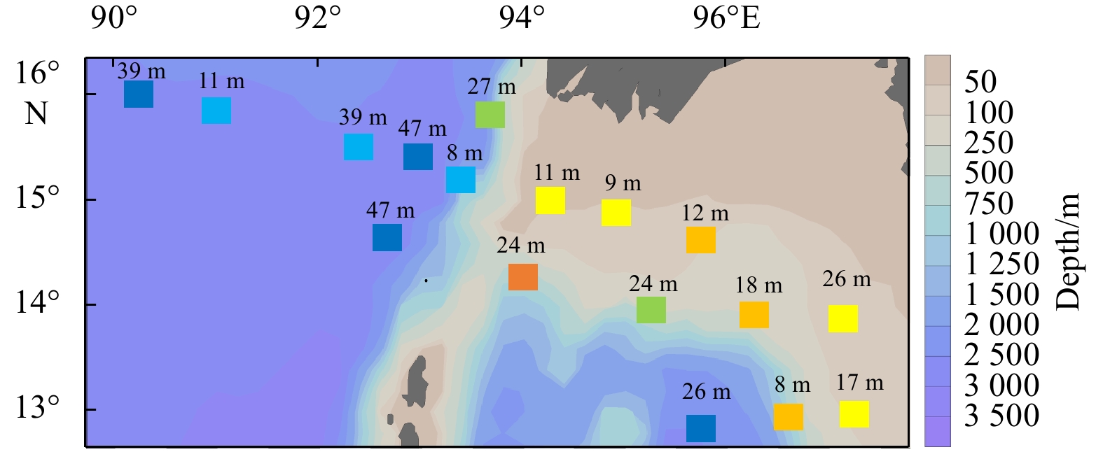
Figure 2. Water depth and mixed layer depth (MLD) measured during the sampling period. The different colors of squares indicate water depths: yellow: 52−79 m, orange: 112−137 m, dark orange: 295 m, green: 639−766 m, blue: 1517−1523 m, dark blue: 2431−2801 m. Numbers above the square indicate MLDs.
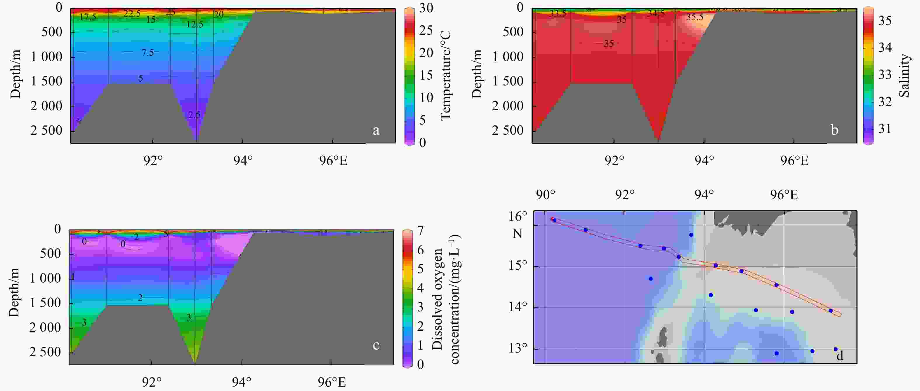
Figure 3. Vertical profiles of temperature (a), salinity (b) and dissolved oxygen concentration (c) of the selected section (d).
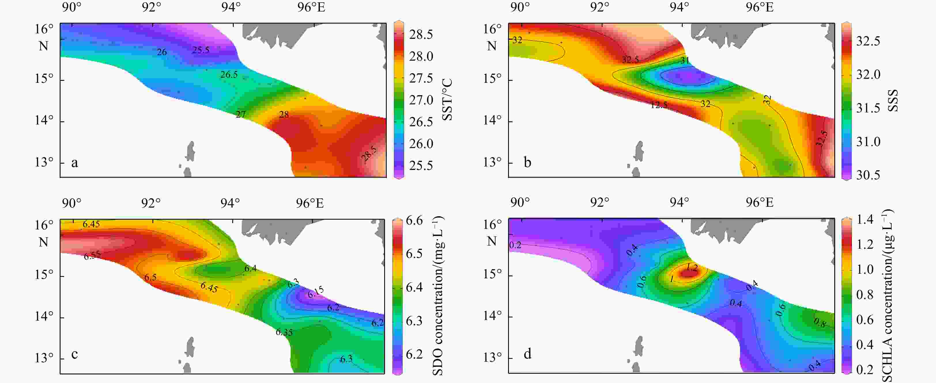
Figure 4. Surface values of temperature (a), salinity (b), dissolved oxygen concentration (c), and chlorophyll a concentration (d). SST: sea surface temperature; SSS: sea surface salinity; SDO: surface dissolved oxygen; SCHLA: surface chlorophyll a.
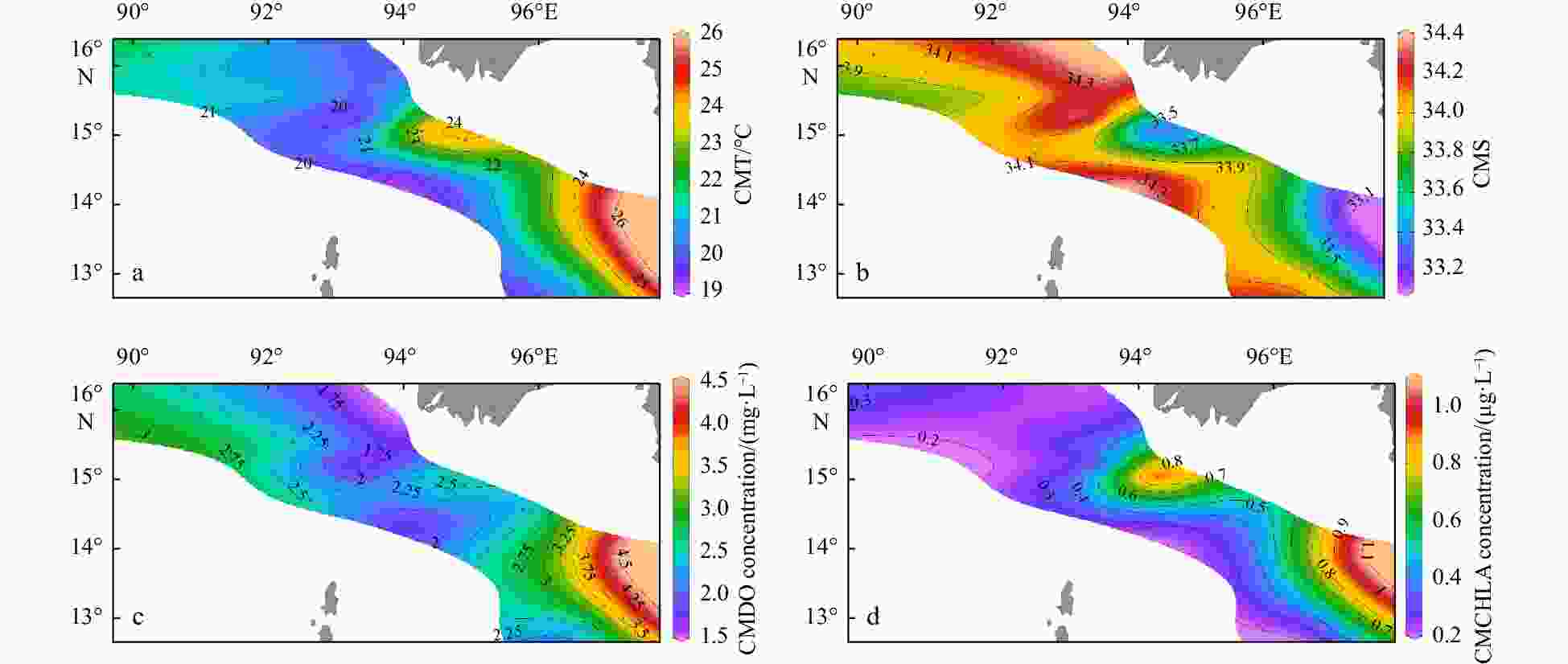
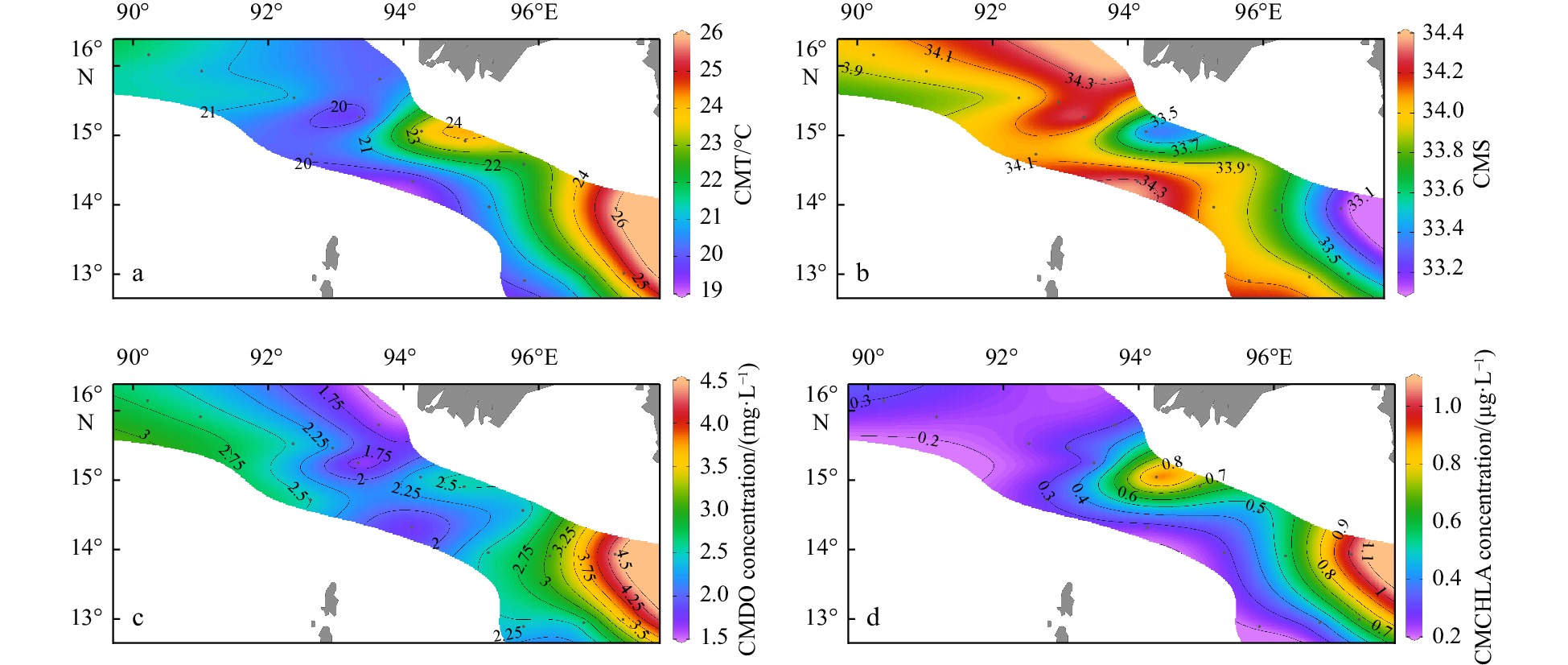
Figure 5. Column mean values of temperature (a), salinity (b), dissolved oxygen concentration (c), and chlorophyll a concentration (d) from 200 m (or the bottom) to the surface. CMT: column mean temperature; CMS: column mean salinity; CMDO: column mean dissolved oxygen; CMCHLA: column mean chlorophyll a.
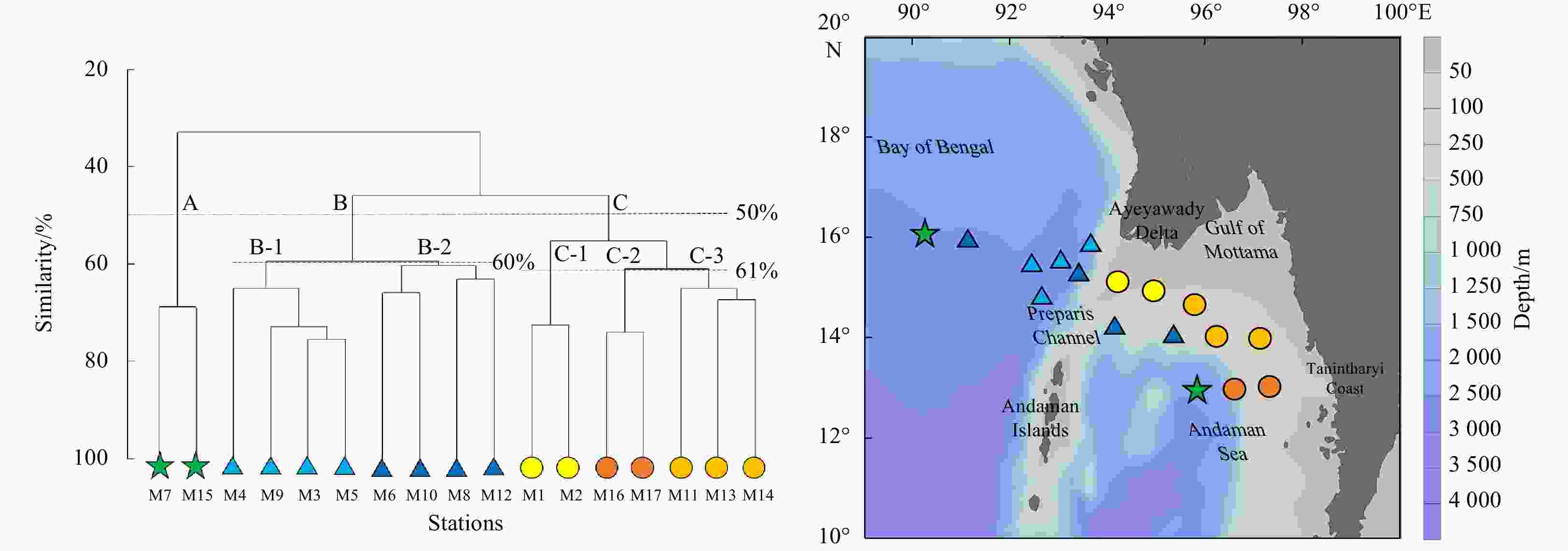
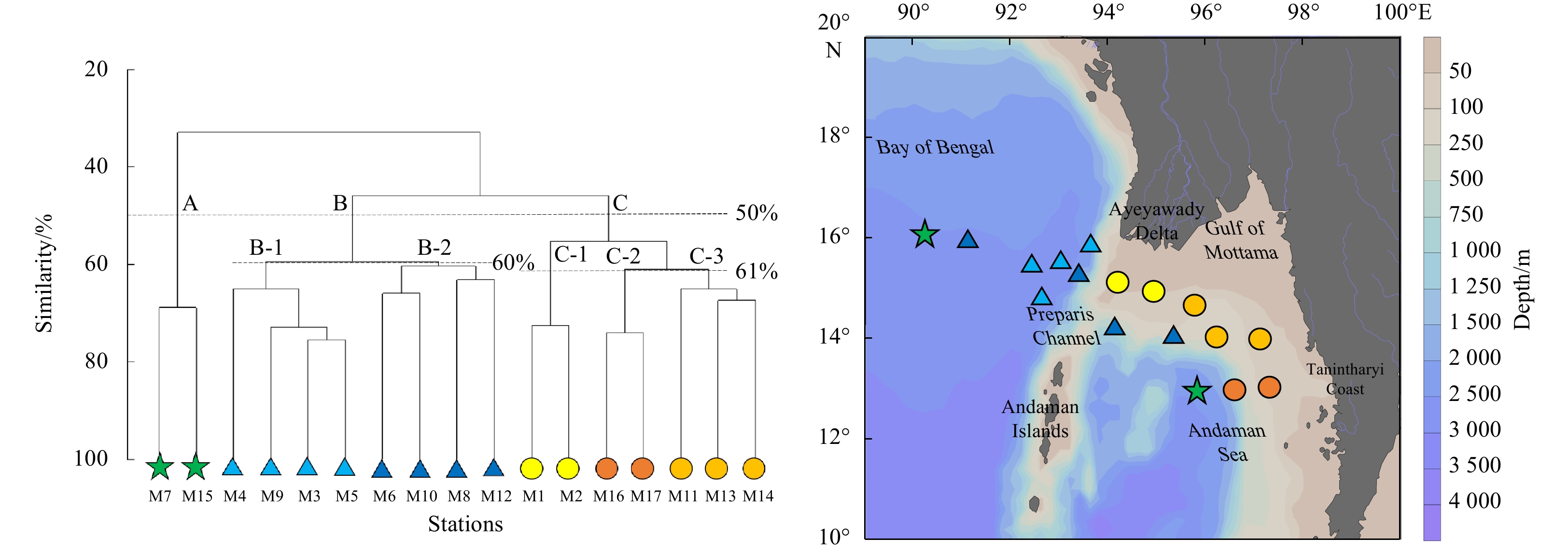
Figure 6. Mesozooplankton community clusters according to taxonomic abundance datasets. Three groups (A: open ocean, B: transition zone, C: nearshore water) were divided at 50% similarity; Group B was divided into two subgroups (B-1 and B-2) at 60% similarity, while Group C was divided into three subgroups (C-1, C-2 and C-3) at 61% similarity. Green stars indicate Group A; light and dark blue triangles indicate Groups B-1 and B-2, respectively; yellow, orange and light orange circles indicate Groups C-1, C-2 and C-3, respectively.

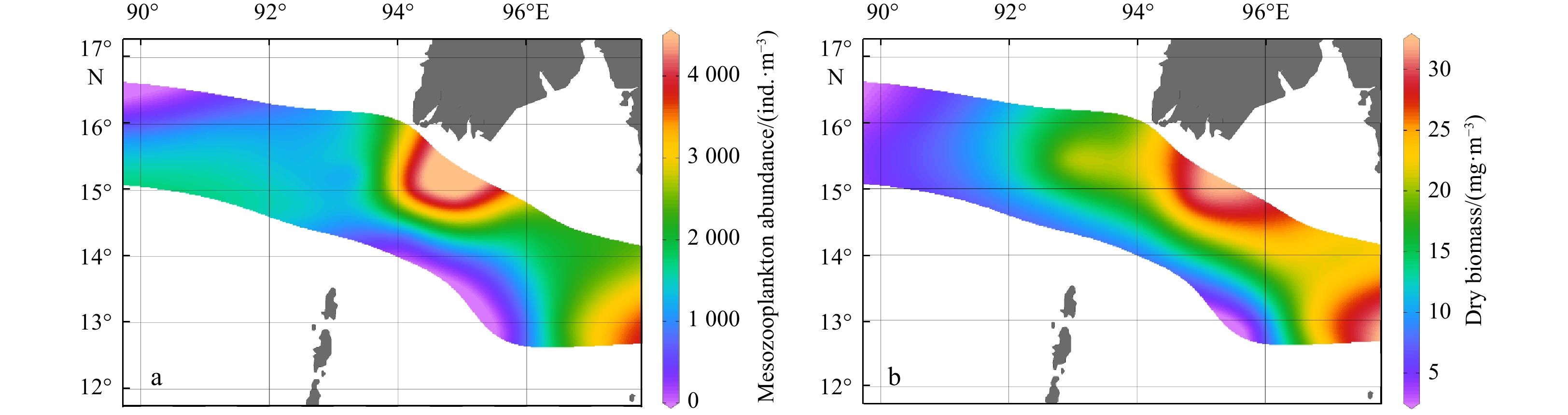
Figure 7. Spatial variations in mesozooplankton abundance (a) and dry biomass (b) in towed water column (200 m or from the bottom to the surface for shallower stations).
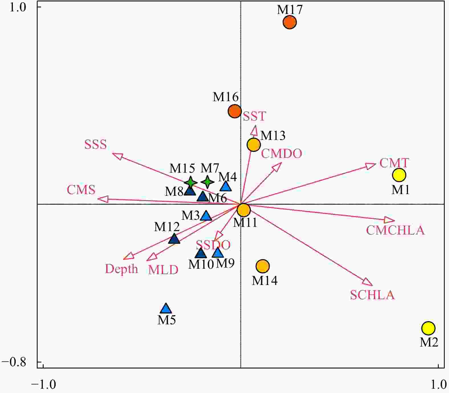
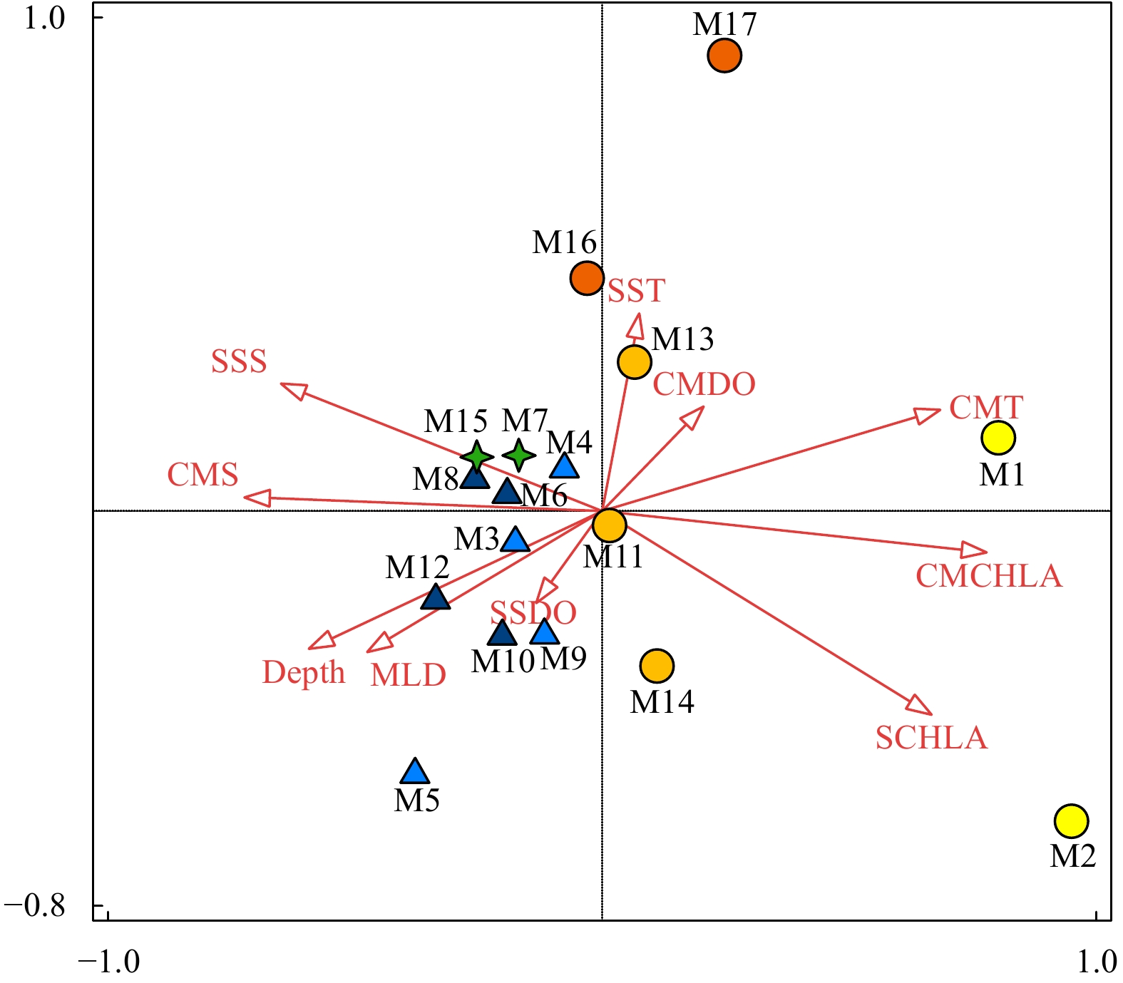
Figure 8. Relationship between ten environmental variables and the mesozooplankton community by interactive-forward-selection RDA. Green stars indicate Group A; light and dark blue triangles indicate Groups B-1 and B-2, respectively; yellow, orange and light orange circles indicate Groups C-1, C-2 and C-3, respectively. MLD: mixed layer depth; SST: sea surface temperature; SSS: sea surface salinity; SDO: surface dissolved oxygen concentration; SCHLA: surface chlorophyll a concentration; CMT: column mean temperature; CMS: column mean salinity; CMDO: column mean dissolved oxygen concentration; CMCHLA: column mean chlorophyll a concentration.

Figure 9. Diagram of “Var-part-3groups-simple-effects-tested-FS” variation partition analysis. a, b, and c represent parts individually controlled by physical, chemical and biological factors, respectively; d represents the part controlled jointly by physical and chemical factors; e represents the part controlled jointly by chemical and biological factors; f represents the part controlled jointly by physical and biological factors; g represents the part controlled by physical, chemical and biological factors collectively. Values under the letters represent explained percentage. Physical factors include depth, mixed layer depth, sea surface temperature, sea surface salinity, column mean temperature, and column mean salinity; chemical factors include surface dissolved oxygen and column mean dissolved oxygen; and biological factors include surface chlorophyll a and column mean chlorophyll a.
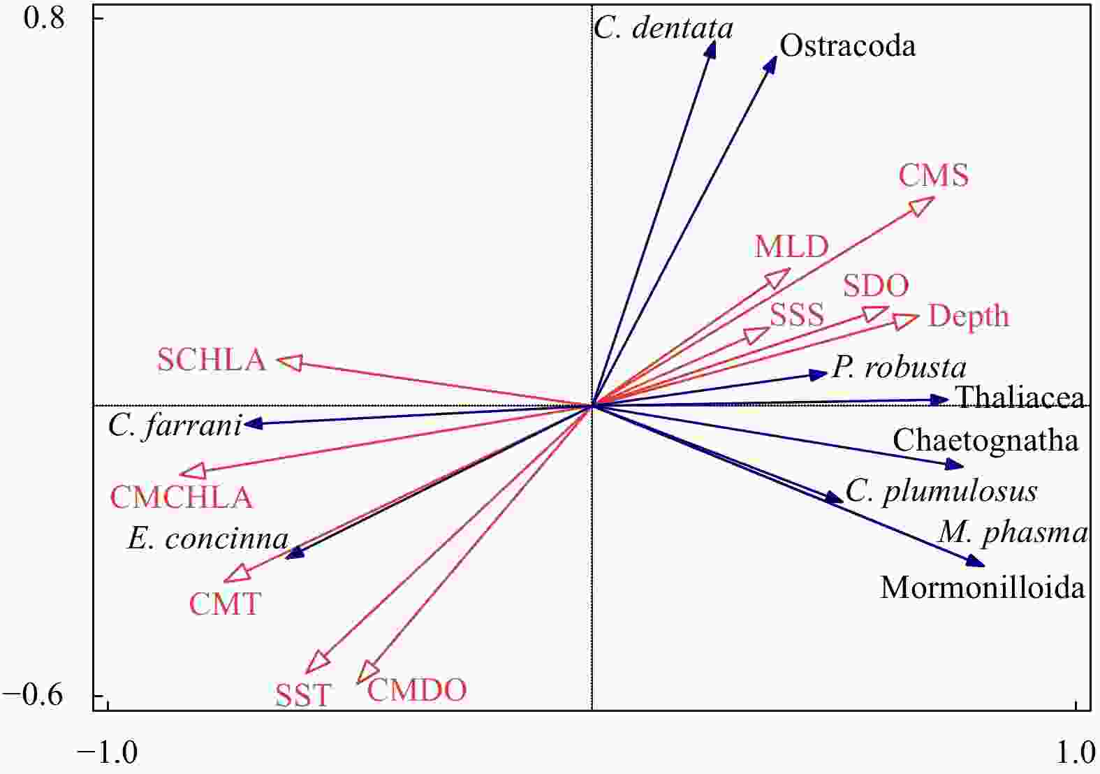
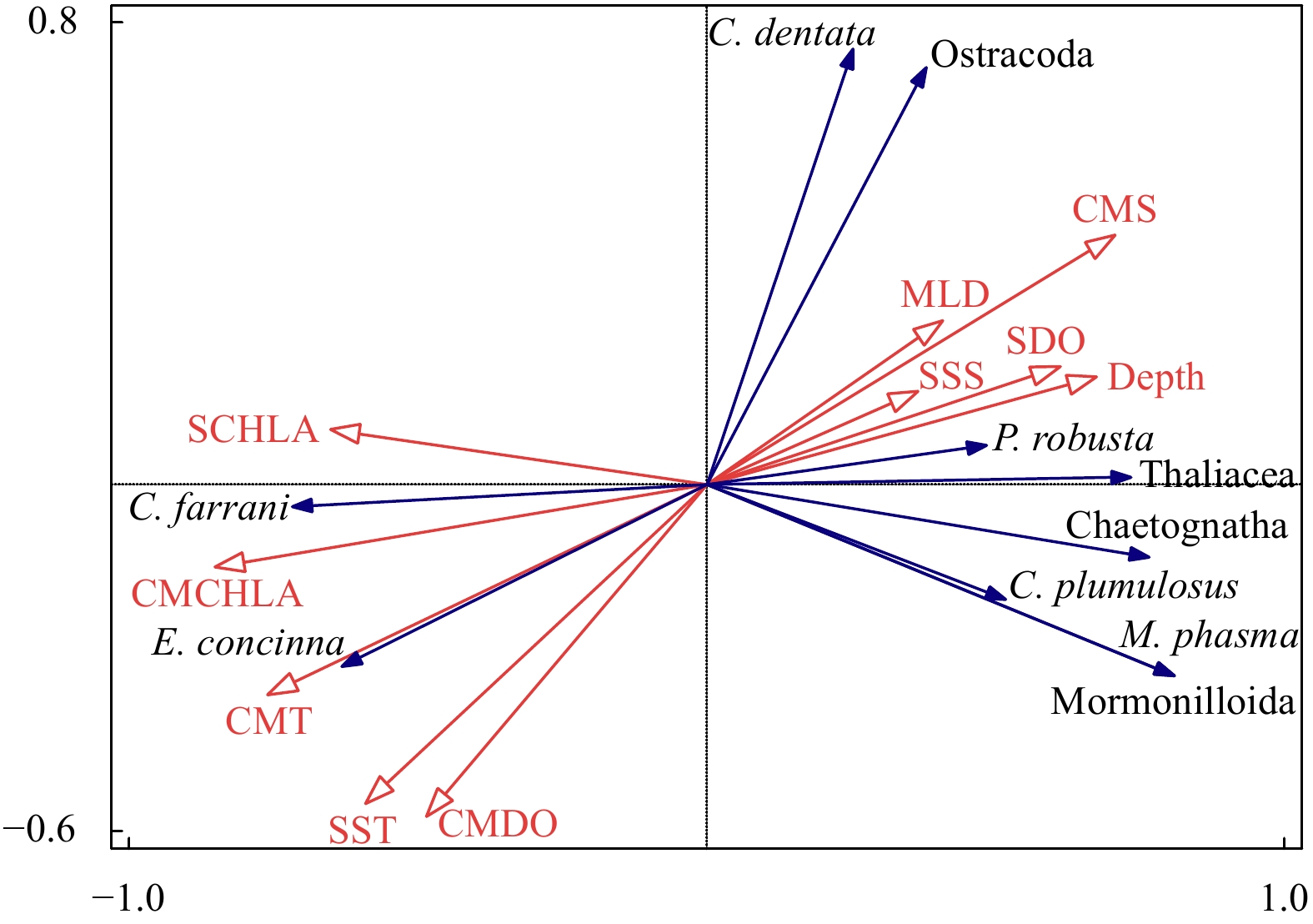
Figure 10. Relationship between ten environmental variables and mesozooplankton taxa by interactive-forward-selection redundancy analysis. C. farrani: Clausocalanus farrani; E. concinna: Euchaeta concinna; C. dentata: Cypridina dentata; P. robusta: Pleuromamma robusta; C. plumulosus: Calocalanus plumulosus; M. phasma: Mormonilla phasma. MLD: mixed layer depth; SST: sea surface temperature; SSS: sea surface salinity; SDO: surface dissolved oxygen concentration; SCHLA: surface chlorophyll a concentration; CMT: column mean temperature; CMS: column mean salinity; CMDO: column mean dissolved oxygen concentration; CMCHLA: column mean chlorophyll a concentration.
Table 1. Spatial variations in mesozooplankton abundance (ind./m3) and dry biomass (mg/m3)
Group Subgroup Abundance in subgroup Dry biomass in subgroup Abundance in groups Dry biomass in groups A − − − 394.7±80.9b 4.0±0.4b B B-1 1519.8±268.7 16.3±4.7 1265.7±343.8b 15.2±4.7b B-2 1011.6±177.2 14.2±5.2 C C-1 4332.7±171.6 26.3±6.2 2958.5±1030.3a 24.8±3.7a C-2 2116.0±298.0 23.6±3.3 C-3 2848.1±481.1 25.0±3.9 Note: Different lowercase letters (a, b) in the same index indicate significant differences among groups (p<0.05). − represents no data.  下载: 导出CSV
Table 2. Spatial variations in the relative abundances (%) of the mesozooplankton taxa
Taxonomic groups Order Differences in Order Differences in Taxonomic groups Group A Group B Group C Group A Group B Group C Subclass Copepoda Calanoida 38.2±0.6 37.3±8.1 44.7±4.7 81.4±7.6 79.9±5.0 85.9±5.7 Cyclopoida 40.2±5.9 39.0±6.5 40.8±8.0 Harpacticoida 0.4±0.1 0.5±0.3 0.3±0.3 >Mormonilloida 2.6±1.2ab 3.2±2.2a 0.1±0.3b Subclass Malacostraca Amphipoda 0.1±0.1 0.2±0.2 0.0±0.1 0.3±0.4 0.6±0.4 0.2±0.3 Mysida 0.0±0.0 0.0±0.0 0.0±0.0 Euphausiacea 0.2±0.3 0.4±0.3 0.1±0.1 Decapoda 0.0±0.0 0.0±0.0 0.0±0.1 Cumacea 0.0±0.0 0.0±0.0 0.0±0.0 Subclass Phyllopoda Cladocera − − − 0.2±0.3 0.1±0.2 0.0±0.0 Subclass Ostracoda − − − − 2.1±0.6ab 3.6±2.6a 0.9±0.6b Class Appendicularia − − − − 8.7±4.7 8.9±3.7 7.6±5.2 Class Thaliacea − − − − 0.5±0.0ab 1.0±0.7a 0.1±0.2b Class Polychaeta − − − − 0.3±0.0 0.2±0.3 0.2±0.3 Phylum Chaetognatha − − − − 1.7±0.8ab 1.9±0.7a 0.8±0.6b Phylum Cnidaria − − − − 0.4±0.1 1.2±0.6 0.4±0.6 Phylum Ctenophora − − − − 0.0±0.0 0.0±0.0 0.0±0.0 Phylum Mollusca − − − − 0.8±0.1 0.3±0.2 0.6±0.7 Phylum Protozoa − − − − 0.5±0.5 0.2±0.2 0.4±0.3 Note: Different lowercase letters (a, b) in the same index indicate significant differences among groups (p<0.05). − represents these taxonomic groups are not subdivided by order.
下载: 导出CSV
Table 3. Spatial variations in the relative abundances (%) of the dominant species
Taxa Dominant species Group A Group B Group C Copepoda Oncaea venusta 23.6±4.2 19.9±6.5 22.9±6.2 Copepoda Oithona spp. 10.6±1.2 12.0±3.0 13.9±5.0 Copepoda Paracalanus aculeatus 10.8±2.6 7.8±3.0 13.8±6.9 Appendicularia Oikopleura spp. 7.7±4.5 8.4±3.5 7.5±5.2 Copepoda Clausocalanus farrani 6.0±0.3ab 3.0±1.6b 6.9±3.0a Copepoda Subeucalanus subtenuis 0.7±0.6 2.3±2.0 3.9±2.9 Copepoda Clausocalanus furcatus 2.9±1.7 5.2±2.5 2.8±2.3 Copepoda Euchaeta larva 1.7±0.0 1.6±0.7 2.7±2.4 Copepoda Clausocalanus/Paracalanus larva 1.4±0.4 2.5±2.0 2.6±2.6 Copepoda Neocalanus larva 2.8±1.0 2.3±1.4 2.5±1.4 Copepoda Acrocalanus gibber 0.9±0.3 1.8±1.0 1.9±1.2 Copepoda Farranula gibbula 2.8±0.1 1.7±1.2 1.4±0.9 Copepoda Triconia conifera 0.7±0.6 2.2±1.3 1.0±0.6 Copepoda Euchaeta concinna 0.7±0.6ab 0.2±0.2b 1.0±0.9a Copepoda Canthocalanus pauper 0.5±0.2 1.2±0.7 1.0±0.8 Copepoda Mormonilla phasma 2.6±1.2ab 3.2±2.2a 0.1±0.3b Ostracoda Cypridina dentata 0.1±0.2ab 1.7±1.9a 0.2±0.3b Copepoda Temora turbinate 0.3±0.4 1.5±1.8 0.6±1.6 Copepoda Scolecithricella nicobarica 0.7±0.6 1.3±0.8 0.7±0.5 Ostracoda Euconchoecia aculeata 0.9±0.1 1.0±0.7 0.5±0.5 Copepoda Corycaeidae larva 0.2±0.2 1.0±0.7 0.5±0.7 Copepoda Calocalanus plumulosus 1.5±0.9a 0.3±0.4ab 0.1±0.2b Planktonic larva Copepoda nauplius larva 1.3±0.6 0.4±0.4 0.9±0.6 Copepoda Pleuromamma robusta 1.0±1.0a 0.3±0.1b 0.1±0.1b Appendicularia Fritillaridae spp. 1.0±0.2 0.5±0.5 0.1±0.1 Chaetognatha Serratosagitta pacifica 1.0±0.6 0.4±0.3 0.5±0.5 Note: Dominant species were defined as having a relative abundance of greater than 1% in at least one group. Different lowercase letters (a, b) in the same index indicate significant differences among groups (p<0.05).
下载: 导出CSV
Table 4. Spatial variations in the environmental variables by the Kruskal–Wallis test
Environmental variables Group A Group B Group C Depth/m 2468.5±53.0a 1473.6±920.3a 89.1±35.0b MLD/m 32.5±9.2 28.4±14.9 14.4±6.3 SST/℃ 27.0±1.5 26.3±0.9 27.6±0.8 SSS 32.1±0.1 32.2±0.5 31.7±0.6 SDO concentration/(mg·L−1) 6.4±0.1 6.5±0.1 6.3±0.1 SCHLA concentration/(µg·L−1) 0.3±0.0 0.4±0.1 0.6±0.3 CMT/℃ 21.0±0.9ab 20.3±0.6b 23.6±1.4a CMS 34.0±0.1a 34.1±0.2a 33.6±0.3b CMDO concentration/(mg·L−1) 2.6±0.2 2.2±0.4 3.0±0.8 CMCHLA concentration/(µg·L−1) 0.3±0.1ab 0.3±0.0b 0.7±0.2a Micro SCHLA/% 7.1 8.5 20.8±8.0 Nano SCHLA/% 15.9 13.7 19.6±5.5 Pico SCHLA/% 77.0 77.7 59.6±11.6 Note: Different lowercase letters (a, b) in the same index indicate significant differences between groups (p<0.05). Size-fractionated chlorophyll a concentrations were measured only at representative stations (M7 in Group A; M9 in Group B; M1, M2, M13, M14 in Group C). A Kruskal–Wallis test was not performed for size-fractionated Chl a. MLD: mixed layer depth; SST: sea surface temperature; SSS: sea surface salinity; SDO: surface dissolved oxygen; SCHLA: surface chlorophyll a; CMT: column mean temperature; CMS: column mean salinity; CMDO: column mean dissolved oxygen; CMCHLA: column mean chlorophyll a. Micro SCHLA, Nano SCHLA and Pico SCHLA represent proportions of micro- (>20 µm), nano- (2−20 µm), and pico- (0.7−2 µm) surface chlorophyll a concentration to total surface chlorophyll a concentration, respectively.
下载: 导出CSV
Table 5. Results of interactive-forward-selection redundancy analyses
Environmental variables Figure 8 Figure 10 Explains/% pseudo-F p p(adj) Explain/% pseudo-F p p(adj) CMCHLA 43.1 11.4 0.006 0.06 30.0 6.4 0.002 0.020 CMDO 12.7 4.0 0.030 0.3 5.2 1.4 0.232 1 CMT 12.6 5.2 0.008 0.08 6.6 1.8 0.148 1 CMS 6.6 3.2 0.030 0.3 10.5 2.5 0.018 0.162 SCHLA 2.6 1.3 0.260 1 5.6 1.6 0.158 1 SDO 2.4 1.2 0.282 1 1.5 0.4 0.822 1 SST 3.6 2.0 0.144 1 8.6 2.2 0.038 0.304 Depth 1.0 0.5 0.662 1 2.2 0.6 0.778 1 SSS 1.2 0.6 0.610 1 3.3 0.9 0.490 1 MLD 0.2 <0.1 0.980 1 5.1 1.6 0.186 1 Note: MLD: mixed layer depth; SST: sea surface temperature; SSS: sea surface salinity; SDO: surface dissolved oxygen concentration; SCHLA: surface chlorophyll a concentration. CMT: column mean temperature; CMS: column mean salinity; CMDO: column mean dissolved oxygen concentration; CMCHLA: column mean chlorophyll a concentration; adj: adjusted.
下载: 导出CSV
Table 6. Species number, abundance, and dry biomass of zooplankton in Indo-Pacific waters
Research area Layer Species number Mesh size Sampling time Abundance/(ind.·m−3) Dry biomass Reference Northern Andaman Sea off Myanmar 0−200 m (or bottom) 213 200 μm February 1916.7
(337.5−4454.0)17.8 mg/m3 (3.7−30.7 mg/m3)
6.1 mg/m3 (in terms of C);
845.7 mg/m2 (in terms of C)this study surface layer − 200 μm Spring 106.1−945.0 4.4−38.6 mg/m3 Jyothibabu et al. (2014) Other Indian waters off North coastal Andhra Pradesh surface layer 112 200 μm January, April, May, November 4473.0 27.8 mg/m3 Rakhesh et al. (2006) off Rushikulya Estuary 0−bottom (<200 m) 93 120 μm January−June 340.0−6550.0 − Mohanty et al. (2010) Kodiakkarai coastal waters surface layer 121 158 μm twelve months − − Damotharan et al. (2010) Open water in Pacific, BOB, and Arabian Sea western boundary currents in the subtropical North Pacific 0−200 m − 160 μm Winter 206.6 (35.1−456.8) − Dai et al. (2016) western tropical
Pacific Ocean0−200 m 259 200 μm Summer 146.7 4.9 mg/m3 Yang et al. (2017) southern BOB 0−200 m 187 505 μm Spring 33.4 − Li et al. (2017) western BOB 0−bottom of thermocline − 200 μm Winter − 777.0 mg/m2 (in terms of C) Jyothibabu et al. (2008) southwestern BOB influenced by a cyclonic eddy mixed layer − 200 μm Winter 760.9 (337.5−4454.0) 35.9 mg/m3 (in terms of C) Jayalakshmi et al. (2015) northern side of cyclonic eddy in central BOB mixed layer − 200 μm Winter 277.0 20.0 mg/m3 (in terms of C) Sabu et al. (2015) western Arabian Sea 0–150 m − 333 μm February 289.9 14.7 mg/m3 (in terms of C) Koppelmann et al. (2003) central Arabian Sea 0–150 m − 333 μm February 371.3 13.1 mg/m3 (in terms of C) Koppelmann et al. (2003) BOB western BOB 0−bottom of thermocline − 200 μm Winter − 777±433 mg/m2 (in terms of C) Jyothibabu et al. (2008) Spring − 223±236 mg/m2 (in terms of C) Jyothibabu et al. (2008) southwestern BOB Summer − 628±499 mg/m2 (in terms of C) Jyothibabu et al. (2008) Winter 70−4288 8.9−35.9 mg/m3 (in terms of C) Jayalakshmi et al. (2015) western BOB mixed layer − 200 μm Spring 2−5340 1.7−162.6 mg/m3 (in terms of C) Fernandes and Ramaiah (2019) Summer 25−4621 1.3–31.0 mg/m3 (in terms of C) Fernandes and Ramaiah (2009) Autumn 100−2482 2.4−53.6 mg/m3 (in terms of C) Fernandes and Ramaiah (2013) Note: Conversion factors for deriving zooplankton carbon biomass from the displacement volume of zooplankton used were as follows: (1) 1 mL zooplankton = 75 mg dry weight; (2) 1 mg dry weight zooplankton = 0.342 mg carbon of zooplankton (Fernandes and Ramaiah, 2009). − represents no data.
下载: 导出CSV
-
Ashjian C J, Campbell R G, Gelfman C, et al. 2017. Mesozooplankton abundance and distribution in association with hydrography on Hanna Shoal, NE Chukchi Sea, during August 2012 and 2013. Deep-Sea Research Part II: Topical Studies in Oceanography, 144: 21–36. doi: 10.1016/j.dsr2.2017.08.012 Cepeda G D, Viñas M D, Molinari G N, et al. 2020. The impact of Río de la Plata plume favors the small-sized copepods during summer. Estuarine, Coastal and Shelf Science, 245: 107000 Chatterjee A, Shankar D, McCreary J P, et al. 2017. Dynamics of Andaman Sea circulation and its role in connecting the equatorial Indian Ocean to the Bay of Bengal. Journal of Geophysical Research: Oceans, 122(4): 3200–3218. doi: 10.1002/2016JC012300 Cornils A, Schnack-Schiel S B, Böer M, et al. 2006. Feeding of Clausocalanids (Calanoida, Copepoda) on naturally occurring particles in the northern Gulf of Aqaba (Red Sea). Marine Biology, 151(4): 1261–1274 Dai Luping, Li Chaolun, Yang Guang, et al. 2016. Zooplankton abundance, biovolume and size spectra at western boundary currents in the subtropical North Pacific during winter 2012. Journal of Marine Systems, 155: 73–83. doi: 10.1016/j.jmarsys.2015.11.004 Damotharan P, Perumal N V, Arumugam M, et al. 2010. Studies on zooplankton ecology from Kodiakkarai (point calimere) coastal waters (south east coast of India). Research Journal of Biological Sciences, 5(2): 187–198. doi: 10.3923/rjbsci.2010.187.198 Domínguez R, Garrido S, Santos A M P, et al. 2017. Spatial patterns of mesozooplankton communities in the northwestern Iberian shelf during autumn shaped by key environmental factors. Estuarine, Coastal and Shelf Science, 198: 257–268 Dur G, Hwang J S, Souissi S, et al. 2007. An overview of the influence of hydrodynamics on the spatial and temporal patterns of calanoid copepod communities around Taiwan. Journal of Plankton Research, 29(S1): i97–i116 Fernandes V. 2008. The effect of semi-permanent eddies on the distribution of mesozooplankton in the central Bay of Bengal. Journal of Marine Research, 66(4): 465–488. doi: 10.1357/002224008787157430 Fernandes V, Ramaiah N. 2009. Mesozooplankton community in the Bay of Bengal (India): spatial variability during the summer monsoon. Aquatic Ecology, 43(4): 951–963. doi: 10.1007/s10452-008-9209-4 Fernandes V, Ramaiah N. 2013. Mesozooplankton community structure in the upper 1, 000 m along the western Bay of Bengal during the 2002 fall intermonsoon. Zoological Studies, 52(1): 31. doi: 10.1186/1810-522X-52-31 Fernandes V, Ramaiah N. 2014. Distributional characteristics of surface-layer mesozooplankton in the Bay of Bengal during the 2005 winter monsoon. Indian Journal of Geo-Marine Sciences, 43(1): 176–188 Fernandes V, Ramaiah N. 2019. Spatial structuring of zooplankton communities through partitioning of habitat and resources in the Bay of Bengal during spring intermonsoon. Turkish Journal of Zoology, 43(1): 68–93. doi: 10.3906/zoo-1805-6 Fernández-Álamo M A, Färber-Lorda J. 2006. Zooplankton and the oceanography of the eastern tropical Pacific: A review. Progress in Oceanography, 69(2–4): 318–359 Fernández De Puelles M L, Molinero J C. 2008. Decadal changes in hydrographic and ecological time-series in the Balearic Sea (western Mediterranean), identifying links between climate and zooplankton. ICES Journal of Marine Science, 65(3): 311–317. doi: 10.1093/icesjms/fsn017 Gomes H R, Goes J I, Saino T. 2000. Influence of physical processes and freshwater discharge on the seasonality of phytoplankton regime in the Bay of Bengal. Continental Shelf Research, 20(3): 313–330. doi: 10.1016/S0278-4343(99)00072-2 Hossain M S, Sarker S, Sharifuzzaman S M, et al. 2020. Primary productivity connects hilsa fishery in the Bay of Bengal. Scientific Reports, 10(1): 5659. doi: 10.1038/s41598-020-62616-5 Irigoien X, Harris R P. 2006. Comparative population structure, abundance and vertical distribution of six copepod species in the North Atlantic: Evidence for intraguild predation?. Marine Biology Research, 2(4): 276–290 Ittekkot V, Nair R R, Honjo S, et al. 1991. Enhanced particle fluxes in Bay of Bengal induced by injection of fresh water. Nature, 351(6325): 385–387. doi: 10.1038/351385a0 Ivanenko V N, Defaye D. 2006. Planktonic deep-water copepods of the family Mormonillidae Giesbrecht, 1893 from the East Pacific Rise (13°N), the Northeastern Atlantic, and near the North Pole (Copepoda, Mormonilloida). Crustaceana, 79(6): 707–726. doi: 10.1163/156854006778026861 Jagadeesan L, Jyothibabu R, Anjusha A, et al. 2013. Ocean currents structuring the mesozooplankton in the Gulf of Mannar and the Palk Bay, southeast coast of India. Progress in Oceanography, 110: 27–48. doi: 10.1016/j.pocean.2012.12.002 Jagadeesan L, Jyothibabu R, Arunpandi N, et al. 2017. Dominance of coastal upwelling over Mud Bank in shaping the mesozooplankton along the southwest coast of India during the Southwest Monsoon. Progress in Oceanography, 156: 252–275. doi: 10.1016/j.pocean.2017.07.004 Jayalakshmi K J, Sabu P, Devi C R A, et al. 2015. Response of micro- and mesozooplankton in the southwestern Bay of Bengal to a cyclonic eddy during the winter monsoon, 2005. Environmental Monitoring and Assessment, 187(7): 473. doi: 10.1007/s10661-015-4609-0 Jeong M K, Suh H L, Soh H Y. 2011. Taxonomy and zoogeography of euchaetid copepods (Calanoida, Clausocalanoidea) from Korean waters, with notes on their female genital structure. Ocean Science Journal, 46(2): 117–132. doi: 10.1007/s12601-011-0011-1 Jyothibabu R, Madhu N V, Maheswaran P A, et al. 2008. Seasonal variation of microzooplankton (20–200 μm) and its possible implications on the vertical carbon flux in the western Bay of Bengal. Continental Shelf Research, 28(6): 737–755. doi: 10.1016/j.csr.2007.12.011 Jyothibabu R, Win N N, Shenoy D M, et al. 2014. Interplay of diverse environmental settings and their influence on the plankton community off Myanmar during the Spring Intermonsoon. Journal of Marine Systems, 139: 446–459. doi: 10.1016/j.jmarsys.2014.08.003 Koppelmann R, Fabian H, Weikert H. 2003. Temporal variability of deep-sea zooplankton in the Arabian Sea. Marine Biology, 142(5): 959–970. doi: 10.1007/s00227-002-0999-y Köster M, Paffenhöfer G A. 2016. How efficiently can doliolids (Tunicata, Thaliacea) utilize phytoplankton and their own fecal pellets?. Journal of Plankton Research, 39(2): 305–315 Li Kaizhi, Yin Jianqiang, Huang Liangmin, et al. 2010. Advances on classification and ecology of pelagic tunicates. Acta Ecologica Sinica (in Chinese), 30(1): 174–185 Li Kaizhi, Yin Jianqiang, Huang Liangmin, et al. 2017. A comparison of the zooplankton community in the Bay of Bengal and South China Sea during April–May, 2010. Journal of Ocean University of China, 16(6): 1206–1212. doi: 10.1007/s11802-017-3229-4 Liao Jiawen, Peng Shiqiu, Wen Xixi. 2020. On the heat budget and water mass exchange in the Andaman Sea. Acta Oceanologica Sinica, 39(7): 32–41. doi: 10.1007/s13131-019-1627-8 Liu Yanliang, Li Kuiping, Ning Chunlin, et al. 2018. Observed seasonal variations of the upper ocean structure and air-sea interactions in the Andaman Sea. Journal of Geophysical Research: Oceans, 123(2): 922–938. doi: 10.1002/2017JC013367 Madhu N V, Jyothibabu R, Maheswaran P A, et al. 2006. Lack of seasonality in phytoplankton standing stock (chlorophyll a) and production in the western Bay of Bengal. Continental Shelf Research, 26(16): 1868–1883. doi: 10.1016/j.csr.2006.06.004 Madhupratap M, Gauns M, Ramaiah N, et al. 2003. Biogeochemistry of the Bay of Bengal: physical, chemical and primary productivity characteristics of the central and western Bay of Bengal during summer monsoon 2001. Deep-Sea Research Part II: Topical Studies in Oceanography, 50(5): 881–896. doi: 10.1016/S0967-0645(02)00611-2 McCreary J P, Kundu P K, Molinari R L. 1993. A numerical investigation of dynamics, thermodynamics and mixed-layer processes in the Indian Ocean. Progress in Oceanography, 31(3): 181–244. doi: 10.1016/0079-6611(93)90002-U Mills C E. 1995. Medusae, siphonophores, and ctenophores as planktivorous predators in changing global ecosystems. ICES Journal of Marine Science, 52(3–4): 575–581 Mohanty A K, Sahu G, Singhsamanta B, et al. 2010. Zooplankton diversity in the nearshore waters of Bay of Bengal, off Rushikulya Estuary. The IUP Journal of Environmental Sciences, 4(2): 61–85 Nuncio M, Kumar S P. 2012. Life cycle of eddies along the western boundary of the Bay of Bengal and their implications. Journal of Marine Systems, 94: 9–17. doi: 10.1016/j.jmarsys.2011.10.002 Paffenhoefer G A, Knowles S C. 1979. Ecological implications of fecal pellet size, production and consumption by copepods. Journal of Marine Research, 37: 35–49 Paffenhöfer G A. 1993. On the ecology of marine cyclopoid copepods (Crustacea, Copepoda). Journal of Plankton Research, 15(1): 37–55. doi: 10.1093/plankt/15.1.37 Prasanna Kumar S, Muraleedharan P M, Prasad T G, et al. 2002. Why is the Bay of Bengal less productive during summer monsoon compared to the Arabian Sea?. Geophysical Research Letters, 29(24): 2235 Prasanna Kumar S, Narvekar J, Nuncio M, et al. 2010. Is the biological productivity in the Bay of Bengal light limited?. Current Science, 98(10): 1331–1339 Prasanna Kumar S, Nuncio M, Narvekar J, et al. 2004. Are eddies nature’s trigger to enhance biological productivity in the Bay of Bengal?. Geophysical Research Letters, 31(7): L07309 Rakhesh M, Raman A V, Sudarsan D. 2006. Discriminating zooplankton assemblages in neritic and oceanic waters: a case for the northeast coast of India, Bay of Bengal. Marine Environmental Research, 61(1): 93–109. doi: 10.1016/j.marenvres.2005.06.002 Ramaswamy V, Gaye B, Shirodkar P V, et al. 2008. Distribution and sources of organic carbon, nitrogen and their isotopic signatures in sediments from the Ayeyarwady (Irrawaddy) continental shelf, northern Andaman Sea. Marine Chemistry, 111(3–4): 137–150 Ramaswamy V, Rao P S, Rao K H, et al. 2004. Tidal influence on suspended sediment distribution and dispersal in the northern Andaman Sea and Gulf of Martaban. Marine Geology, 208(1): 33–42. doi: 10.1016/j.margeo.2004.04.019 Rao P S, Ramaswamy V, Thwin S. 2005. Sediment texture, distribution and transport on the Ayeyarwady continental shelf, Andaman Sea. Marine Geology, 216(4): 239–247. doi: 10.1016/j.margeo.2005.02.016 Rodolfo K S. 1969. Sediments of the Andaman Basin, northeastern Indian Ocean. Marine Geology, 7(5): 371–402. doi: 10.1016/0025-3227(69)90014-0 Sabu P, Devi C R A, Lathika C T, et al. 2015. Characteristics of a cyclonic eddy and its influence on mesozooplankton community in the northern Bay of Bengal during early winter monsoon. Environmental Monitoring and Assessment, 187(6): 330. doi: 10.1007/s10661-015-4571-x Schott F A, McCreary J P. 2001. The monsoon circulation of the Indian Ocean. Progress in Oceanography, 51(1): 1–123. doi: 10.1016/S0079-6611(01)00083-0 Shankar D, Vinayachandran P N, Unnikrishnan A S. 2002. The monsoon currents in the north Indian Ocean. Progress in Oceanography, 52(1): 63–120. doi: 10.1016/S0079-6611(02)00024-1 Skjoldal H R, Wiebe P H, Postel L, et al. 2013. Intercomparison of zooplankton (net) sampling systems: results from the ICES/GLOBEC sea-going workshop. Progress in Oceanography, 108: 1–42. doi: 10.1016/j.pocean.2012.10.006 Šmilauer P, Lepš J. 2014. Multivariate analysis of ecological data using Canoco 5, second edition. Cambridge, UK: Cambridge University Press, 362 Srichandan S, Baliarsingh S K, Prakash S, et al. 2018. Zooplankton research in Indian seas: a review. Journal of Ocean University of China, 17(5): 1149–1158. doi: 10.1007/s11802-018-3463-4 Steinberg D K, Lomas M W, Cope J S. 2012. Long-term increase in mesozooplankton biomass in the Sargasso Sea: linkage to climate and implications for food web dynamics and biogeochemical cycling. Global Biogeochemical Cycles, 26(1): GB1004 Subramanian V. 1993. Sediment load of Indian Rivers. Current Science, 64(11–12): 928–930 Yang Guang, Li Chaolun, Wang Yanqing, et al. 2017. Spatial variation of the zooplankton community in the western tropical Pacific Ocean during the summer of 2014. Continental Shelf Research, 135: 14–22. doi: 10.1016/j.csr.2017.01.009 Yuan L L, Pollard A I. 2018. Changes in the relationship between zooplankton and phytoplankton biomasses across a eutrophication gradient. Limnology and Oceanography, 63(6): 2493–2507. doi: 10.1002/lno.10955 -


 点击查看大图
计量
- 文章访问数: 388
- HTML全文浏览量: 135
- PDF下载量: 25
- 被引次数: 0