

Parameterization, Sensitivity, and Uncertainty of 1-D Thermodynamic Thin-ice Thickness Retrieval
-
Abstract: Retrieval of thin-ice thickness (TIT) using thermodynamic modeling is sensitive to the parameterization of the independent variables (coded in the model) and the uncertainty of the measured input variables. This article examines the deviation of the classical model’s TIT output when using different parameterization schemes and the sensitivity of the output to the ice thickness. Moreover, it estimates the uncertainty of the output in response to the uncertainties of the input variables. The parameterized independent variables include atmospheric longwave emissivity, air density, specific heat of air, latent heat of ice, conductivity of ice, snow depth, and snow conductivity. Measured input parameters include air temperature, ice surface temperature, and wind speed. Among the independent variables, the results show that the highest deviation is caused by adjusting the parameterization of snow conductivity and depth, followed ice conductivity. The sensitivity of the output TIT to ice thickness is highest when using parameterization of ice conductivity, atmospheric emissivity, and snow conductivity and depth. The retrieved TIT obtained using each parameterization scheme is validated using in situ measurements and satellite-retrieved data. From in situ measurements, the uncertainties of the measured air temperature and surface temperature are found to be high. The resulting uncertainties of TIT are evaluated using perturbations of the input data selected based on the probability distribution of the measurement error. The results show that the overall uncertainty of TIT to air temperature, surface temperature, and wind speed uncertainty is around 0.09 m, 0.049 m, and −0.005 m, respectively.
-

Figure 1. The geographic locations of (a) the sonar sites, (b) the IceBridge footprints, (c) the IABP buoys, and (d) the wind speed stations used in this study.

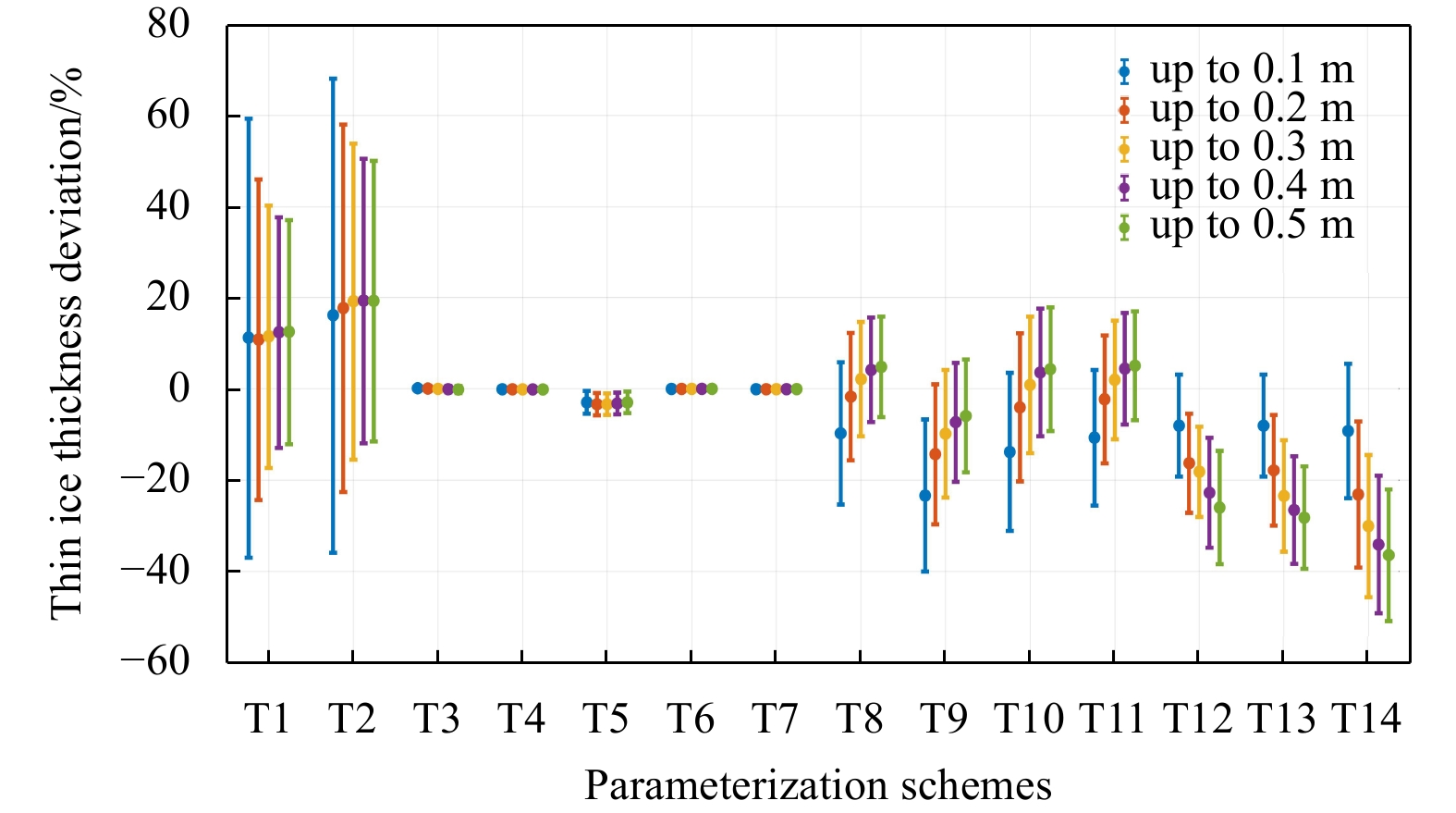
Figure 3. The relative deviation of the model output TIT using each test scheme (T1, T2, … T14) from the TIT obtained using the default scheme. The solid points are mean values of the deviation, and the vertical lines represent one standard deviation. The colors denote the upper limit of the different TIT bins, from 0.1 m to 0.5 m.
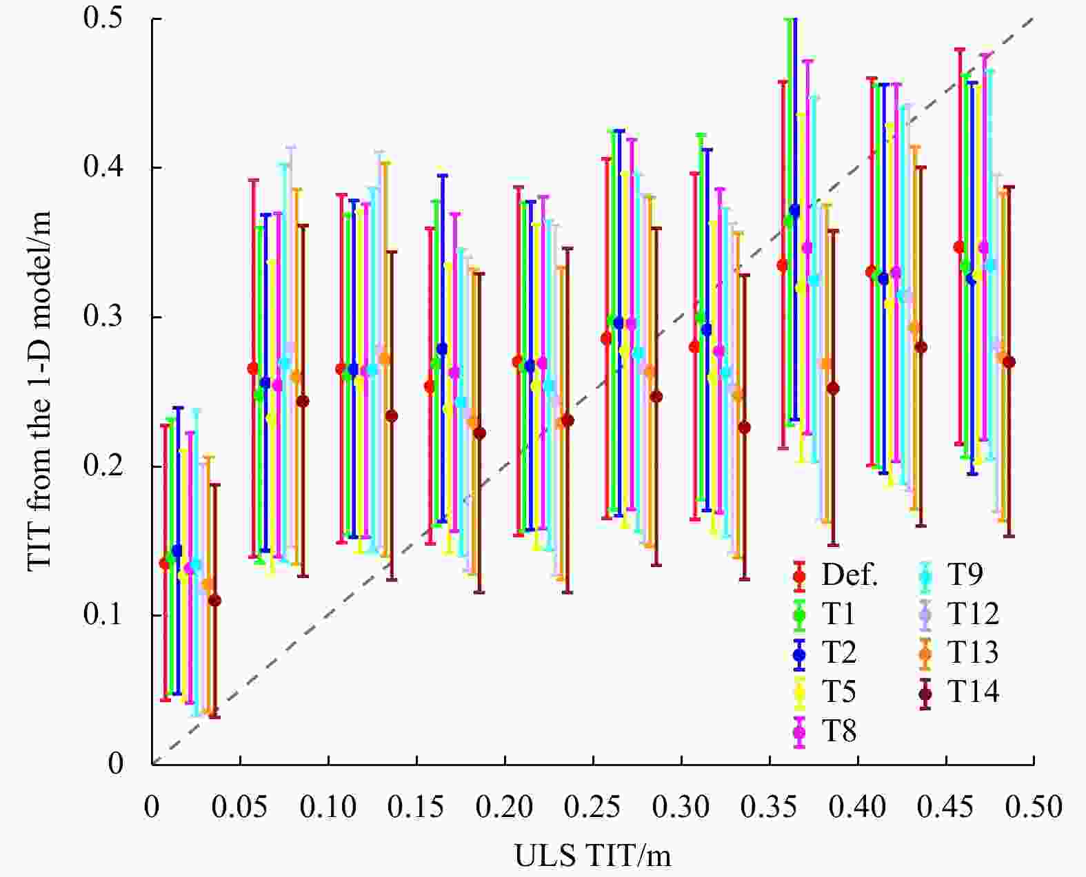
Figure 4. TIT from the 1-D model versus the ULS data, obtained for different TIT intervals. The solid dots represent the mean value from the model, and the error bars represent 0.5 standard deviation.
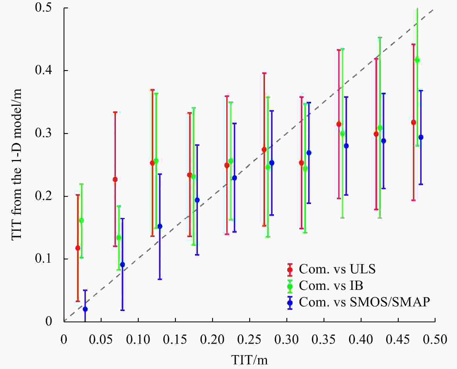
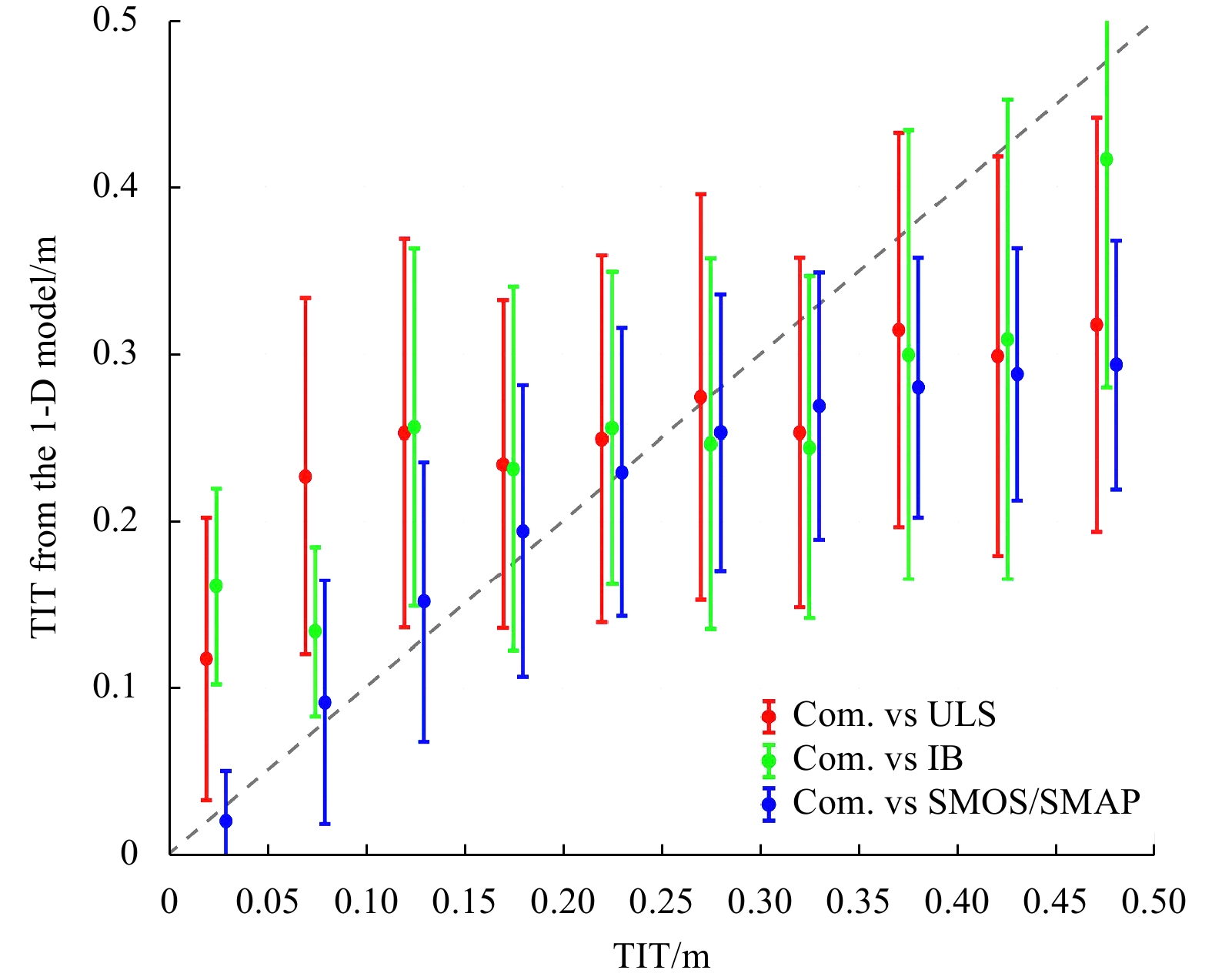
Figure 5. Comparison between the model-retrieved TIT using the combination of schemes T5 and T9 and the TIT from the ULS, IceBridge (IB), and SMOS/SMAP products, respectively. The Cmb. denotes the combination scheme. The interval between the data on the horizontal scale is 0.05 m. The error bars represent 0.5 standard deviation.

Figure 6. Comparisons of (a) ERA5
$ {T}_{a} $ versus IABP$ {T}_{a} $ , (c) MODIS$ {T}_{s} $ versus IABP$ {T}_{s} $ , and (e) ERA5$ u $ versus NWS-observed$ u $ , and their corresponding probability distributions of the differences in (b), (d) and (f), respectively, with fitted curves (black lines). The error bars represent one standard deviation. The numbers between brackets in (a) and (e) denote the data counts. Fig.s (a) and (c) share the same data counts. The numbers in (b), (d), and (f) at the peak of each curve are the mean value of the differences.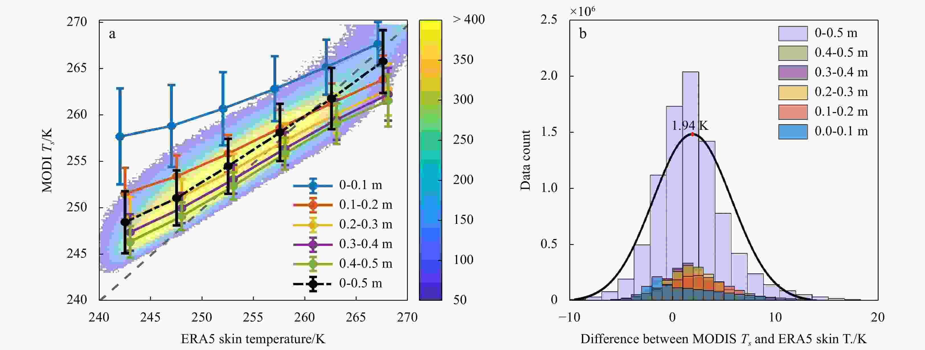
Figure 7. (a) Plot between
$ {T}_{s} $ from MODIS and ERA5. (b) Histogram of the difference between the measurements. The shadow colors in (a) show the counts of data. The error bars represent one standard deviation. The black lines in (b) are the fitted Gaussian curves, and the number at the peak is the mean difference.
Figure 8. Plots showing the retrieved TIT obtained using the original
$ {T}_{s} $ ,$ {T}_{a} $ , and$ u $ as inputs (values in the horizontal axis) and the retrieved TIT with perturbations added representing the error in measurements from (a)$ {T}_{a} $ (with respect to IABP$ {T}_{a} $ ), (b)$ {T}_{s} $ (with respect to IABP$ {T}_{s} $ ) , (c)$ {T}_{s} $ (with respect to ERA5 skin temperature), and (d)$ u $ (with respect to the NWS/NDBC observations). The error bars represent one standard deviation. The shadow colors show the counts of the data points.Table 1. Summary of the previous uncertainty in TIR-TIT retrieval. The symbols are specified in the symbol list of Appendix 2. The data sources of AVHRR or MODIS are used for
$ {T}_{s} $ , and the National Centers for Environmental Prediction (NCEP), High Resolution Limited Area Model (HIRLAM), or ERA-Interim reanalysis data are the other meteorological input variables of the 1-D model. In the third column, the green color denotes the analysis scheme for the errors in the input variables, the values on the right side of the positive and negative signs ‘±’ are the analyzed variable’s errors, and the blue color is for comparing the sources of the different input variables.Reference Data source (data volume) Uncertainty analysis scheme Findings (Yu and Rothrock, 1996) AVHRR (13 images) $ {T}_{s} $ ± 1 K, $ {T}_{a} $ ± 1.6 K,
$ u $ ± 2 m/s1. The uncertainty of the TIT caused by the error in the variables increases with the ice thickness.
2. The uncertainty of the cumulative distribution is no more than 3% for ice thinner than 0.2 m.(Willmes et al., 2010) AVHRR + NCEP (1 image) $ {T}_{a} $ ± 5 K, $ u $ ± 3 m/s Results in max. TIT errors of ±20% (for TIT ≤ 0.5 m) (Wang et al., 2010) MODIS (case study) $ {T}_{s} $ ± 2 K, $ u $ ± 1 m/s For TIT < 0.3 m, TIT is −0.172 m or +0.179 m when $ {T}_{s} $+ 2 K or −2 K; TIT is +0.166 m or −0.133 m when $ u $+1 m/s or −1 m/s. (Mäkynen et al., 2013) MODIS + HIRLAM
(199 images)– The largest TIT uncertainty comes from air temperature. (Adams et al., 2013) MODIS + NCEP / COSMO (two-winter data) $ {T}_{s} $ ± 1.6 K, $ {T}_{a} $ ± 4.5 K;
$ u $ ± 1.3 m/s, NCEP vs COSMO1. For all the variables’ uncertainties, the TIT varies by ±0.37 m for TIT of ≤ 0.5 m.
2. The NCEP $ {T}_{a} $ leads to overestimated ice thicknesses, in comparison to COSMO $ {T}_{a} $.(Zeng et al., 2016) MODIS + ERA-Interim
(four images)Altering the value of $ {T}_{a}-{T}_{s} $ 1. For $ {T}_{a}-{T}_{s} $ > +3 K, the $ {T}_{a}-{T}_{s} $ error of only +1 K causes the TIT to vary by +0.1 m.
2. For $ {T}_{a}-{T}_{s} $ ≤ 0 K or > +2 K, the TIT decreases by 1 to 2 cm or 9 cm when U increases from 0 m/s to 12 m/s. 下载: 导出CSV
Table 2. The specifications of the sonar measurements used in this study
Data source Data form Number of sites Data period Number of samples Nominal error (cm) NPEO 10-min ice draft data 2 2002, 2005 10 10 BGEP Daily average draft statistics 34 2003–2021 737 5–10 IOS-EBS 4-min ice draft data 1 2003 1724 5 IOP 5-min ice draft data 5 2005–2008 3305 10 Note: NPEO is the abbreviation for the North Pole Environmental Observatory (Morison, 2009). BGEP denotes the Beaufort Gyre Exploration Project. IOS and EBS are the short forms for the Institute of Ocean Sciences and the Eastern Beaufort Sea, respectively (Melling and Riedel, 2008). IOP denotes the Integrative Observational Platforms from the University of Washington.
下载: 导出CSV
Table 3. The station ID and geographic locations of the wind speed observation stations
Data source Station ID Longitude, latitude Temporal resolution NWS 99950 −8.46, 71.0 1 hour 99710 19.00, 74.50 99720 25.01, 76.51 99740 28.89, 78.91 99752 16.54, 76.47 99790 13.63, 78.07 99927 16.24, 80.06 99935 25.00, 80.65 99938 31.46, 80.10 NDBC ULRA2 −160.78, 63.87 6 min PRDA2 −148.53, 70.40
下载: 导出CSV
Table 4. The parameterized variable test schemes. All the symbols and equations in the third and fourth columns are introduced in Appendix 1.
Test scheme no. Parameter Default scheme Parameterization scheme
(equation name / equation number)T1 Atmospheric emissivity ($ {\varepsilon }_{a} $) $ {\varepsilon }_{a\_\mathrm{J}\mathrm{X}06} $ (+$ {\mathrm{E}}_{\mathrm{A}\mathrm{E}96}^{\mathrm{\text{'}}} $) $ {\varepsilon }_{a\_\mathrm{E}\mathrm{F}61}(+{\mathrm{E}}_{\mathrm{A}\mathrm{E}96}^{\mathrm{\text{'}}}) $ Eq. A1 (+ Eq. A6) T2 $ {\varepsilon }_{a\_\mathrm{K}\mathrm{L}94} $ Eq. A2 T3 $ {\varepsilon }_{a\_\mathrm{J}\mathrm{X}06} $ (+$ {\mathrm{E}}_{\mathrm{M}78} $) (denoted as $ {\varepsilon }_{a\_J/M} $) Eq. A3 (+ Eq. A4) T4 $ {\varepsilon }_{a\_\mathrm{J}\mathrm{X}06} $ (+$ {\mathrm{E}}_{\mathrm{A}\mathrm{E}96} $) ($ {\varepsilon }_{a\_J/A} $) Eq. A3 (+ Eq. A5) T5 Air density ($ {\rho }_{a} $, $ \mathrm{k}\mathrm{g}/{\mathrm{m}}^{3} $) $ {\rho }_{a}=1.3 $ $ {\rho }_{a\_GL} $ Eq. A7 T6 Specific heat of air ($ {c}_{p} $, $ \mathrm{J}/(\mathrm{k}\mathrm{g}\cdot\mathrm{K}) $) $ {c}_{p}= $1004 $ {\mathrm{c}}_{\mathrm{p}\mathrm{w}} $ Eq. A8 T7 Latent heat of sublimation ($ {L}_{s} $,$ \mathrm{J}/\mathrm{k}\mathrm{g} $) $ {L}_{s}=2.5\times {10}^{6} $ $ {L}_{sw} $ Eq. A9 T8 Ice conductivity ($ {k}_{i} $, $ \mathrm{W}/(\mathrm{m}\cdot\mathrm{K}) $) $ {k}_{i}=2.03 $ $ {k}_{i\_\mathrm{U}64} $ (+$ {k}_{0\_\mathrm{N}64}+{S}_{i\_\mathrm{J}94} $) ($ {k}_{i\_UNJ} $) Eq. A10 (+Eq. A11 + Eq. A15) T9 $ {k}_{i\_\mathrm{U}64} $ (+$ {k}_{0\_\mathrm{S}78}+{S}_{i\_\mathrm{J}94} $) ($ {k}_{i\_USJ} $) Eq. A10 (+Eq. A12 + Eq. A15) T10 $ {k}_{i\_\mathrm{U}64} $ (+$ {k}_{0\_\mathrm{C}10}+{S}_{i\_\mathrm{J}94} $) ($ {k}_{i\_UCJ} $) Eq. A10 (+Eq. A13 + Eq. A15) T11 $ {k}_{i\_\mathrm{U}64} $ (+$ {k}_{0\_\mathrm{C}10}+{S}_{i\_\mathrm{C}74} $) ($ {k}_{i\_UCC} $) Eq. A10 (+Eq. A13 + Eq. A14) T12 Snow depth ($ {h}_{s} $, m) $ {h}_{s}=0 $ $ {h}_{s\_\mathrm{D}71}(+{k}_{s1}) $ Eq. A16 T13 $ {h}_{s\_\mathrm{M}19}(+{k}_{s1}) $ Eq. A17 T14 Snow conductivity ($ {k}_{s} $, $ \mathrm{W}/(\mathrm{m}\cdot\mathrm{K}) $) $ {k}_{s1}=0.33 (+{h}_{s\_M19}) $ $ {k}_{s2}=0.21(+{h}_{s\_\mathrm{M}19}) $ (+ Eq. A17)
下载: 导出CSV
Table 5. The mean deviation of TIT (in %) for the 14 parameterization schemes with respect to the default scheme. Calculations are for the three shown ice thickness bins as well as the average TIT over the entire thickness range of 0–0.5 m.
Test scheme 0.0–0.1 m 0.2–0.3 m 0.4–0.5 m 0–0.5 m T1 11.18 12.81 14.34 12.49 T2 16.11 22.20 17.20 19.25 T3 0.10 −0.15 −0.46 −0.16 T4 −0.10 −0.14 −0.20 −0.14 T5 −2.99 −3.40 −1.92 −3.00 T6 −0.03 −0.01 0.00 −0.01 T7 −0.09 −0.08 −0.02 −0.07 T8 −9.77 9.31 10.50 4.79 T9 −23.40 −1.40 0.95 −5.95 T10 −13.84 10.09 11.65 4.29 T11 −10.72 9.93 11.70 5.05 T12 −8.09 −23.52 −38.09 −26.02 T13 −8.09 −33.34 −35.63 −28.23 T14 −9.25 −41.79 −46.52 −36.44
下载: 导出CSV
Table 6. The sensitivity of the model’s output to increments in TIT of 0.1 m for the 14 parameterization equation schemes
Test scheme Sensitivity (%) Test scheme Sensitivity (%) T1 0.33 T8 3.64 T2 0.79 T9 4.36 T3 −0.07 T10 4.53 T4 −0.01 T11 3.94 T5 0.00 T12 −4.48 T6 0.00 T13 −5.03 T7 0.00 T14 −6.80
下载: 导出CSV
Table 7. The deviation (in percentage) of the model TIT with respect to the ULS TIT based on the different parameterization schemes. The deviation was calculated according to Eq. (7) in Section 3.
Scheme Ice bin (cm) 0–5 5–10 10–15 15–20 20–25 25–30 30–35 35–40 40–45 Def. 9.35 1.92 0.94 0.28 0.06 −0.04 −0.25 −0.18 −0.32 T1 10.65 2.43 1.05 0.39 0.16 0.00 −0.18 −0.13 −0.25 T2 10.21 2.13 1.02 0.48 0.14 0.05 −0.11 −0.05 −0.25 T5 10.73 2.27 1.02 0.54 0.15 0.04 −0.14 −0.03 −0.26 T8 9.62 1.99 0.98 0.31 0.09 −0.03 −0.23 −0.17 −0.30 T9 10.59 2.28 1.04 0.45 0.16 0.04 −0.17 −0.09 −0.24 T12 10.38 2.48 1.04 0.33 0.09 −0.03 −0.23 −0.16 −0.28 T13 10.17 2.64 1.18 0.28 0.02 −0.08 −0.25 −0.31 −0.29 T14 10.40 2.36 1.11 0.24 −0.04 −0.09 −0.27 −0.31 −0.34
下载: 导出CSV
Table 8. Statistics of the difference between the model and ULS TIT based on the different parameterization schemes.
Scheme Bias (m) RMSE (m) MAE (m) $ {\mathrm{R}}^{2} $ $ \rho $ Def. 0.027 0.103 0.088 0.741 0.861 T1 0.031 0.101 0.086 0.766 0.875 T2 0.032 0.106 0.089 0.693 0.832 T5 0.010 0.100 0.087 0.766 0.875 T8 0.028 0.101 0.088 0.755 0.869 T9 0.018 0.106 0.091 0.663 0.814 T12 0.004 0.120 0.102 0.367 0.606 T13 −0.004 0.120 0.102 0.407 0.638 T14 −0.018 0.118 0.102 0.511 0.715 *footnote: RMSE = root-mean-square error, MAE = mean absolute error, $ {R}^{2} $ is the coefficient of determination, $ \rho $ is the Pearson’s linear correlation coefficient. The p-value of rho for each scheme is no more than 0.05.
下载: 导出CSV
Table 9. Bias of
$ {T}_{a} $ (ERA5 minus IABP measurements) and$ {T}_{s} $ (MODIS minus IABP) for the different ice bins and temperature bins. Correlation coefficients$ \rho $ of the data from the two sources are also shown.Ice bin (m) Bias for different temperature bins (K) Bias (K) $ \rho $ 240–245 245–250 250–255 255–260 260–265 265–270 $ {T}_{a} $ 0.0–0.1 - −2.08 −1.17 −1.96 −2.84 −3.59 −2.24 0.86 0.1–0.2 - −1.28 −2.68 −2.64 −4.91 −4.23 −3.19 0.81 0.2–0.3 6.62 −0.95 −4.01 −3.39 −5.53 −4.59 −3.81 0.82 0.3–0.4 3.42 −2.25 −3.39 −4.92 −5.93 −4.98 −3.80 0.76 0.4–0.5 3.77 −3.13 −3.36 −5.41 −5.57 −4.45 −4.05 0.71 0.0–0.5 4.06 −2.11 −3.36 −3.87 −5.31 −4.44 −3.62 0.75 $ {T}_{s} $ 0.2–0.3 5.71 3.94 −0.50 −3.69 - - −0.57 0.47 0.3–0.4 5.43 −0.02 −0.62 −5.13 - - −1.67 0.61 0.4–0.5 3.16 −0.90 −0.59 −6.54 - - −3.78 0.62 0.0–0.5 4.72 0.89 0.08 −3.88 - - −1.38 0.53
下载: 导出CSV
Table 10. Statistics of the difference between ERA5
$ u $ and the observed$ u $ for different ice bins and wind speed binsIce bin (m) Bias for different wind speed bins (m/s) Bias (m/s) $ \rho $ 0–5 5–10 10–15 15–20 $ u $ 0.0–0.1 0.93 −1.1 −3.61 −5.12 −1.17 0.65 0.1–0.2 1.16 −0.3 −3.76 −4.74 0.07 0.68 0.2–0.3 0.99 −0.54 −2.67 −4.95 −0.15 0.74 0.3–0.4 0.81 −0.94 −3.13 −5.71 −0.41 0.72 0.4–0.5 0.65 −0.99 −4.48 −3.80 −0.35 0.69 0.0–0.5 0.94 −0.93 −3.54 −5.07 −0.75 0.68
下载: 导出CSV
Table 11. The uncertainty (bias, m) of TIT due to the uncertainty of the input variables of
$ {T}_{a} $ ,$ {T}_{s} $ , and$ u $ . Columns 2–5 correspond to the uncertainty of the input variables in Fig.s 6b, 6d, 6f, and 7b.Ice bin (m) $ {T}_{a} $ $ {T}_{s}(\mathrm{v}\mathrm{s}.\mathrm{ }\mathrm{I}\mathrm{A}\mathrm{B}\mathrm{P}) $ $ {T}_{s}(\mathrm{v}\mathrm{s}.\mathrm{ }\mathrm{E}\mathrm{R}\mathrm{A}5) $ $ u $ 0–0.1 0.047 −0.027 0.068 0.000 0.1–0.2 0.117 −0.100 0.088 −0.002 0.2–0.3 0.127 −0.178 0.065 −0.006 0.3–0.4 0.104 −0.261 0.017 −0.009 0.4–0.5 0.064 −0.346 −0.045 −0.010 0–0.5 0.090 −0.200 0.049 −0.005
下载: 导出CSV
-
Adams S, Willmes S, Schröder D, et al. 2012. Daily thin-ice thickness maps from modis thermal infrared imagery. In: 2012 IEEE International Geoscience and Remote Sensing Symposium. Munich: IEEE, 3265–3268. Adams S, Willmes S, Schröder D, et al. 2013. Improvement and sensitivity analysis of thermal thin-ice thickness retrievals. IEEE Transactions on Geoscience and Remote Sensing, 51(6): 3306–3318. doi: 10.1109/TGRS.2012.2219539 Alduchov O A, Eskridge R E. 1996. Improved magnus form approximation of saturation vapor pressure. Journal of Applied Meteorology, 35(4): 601–609. doi: 10.1175/1520-0450(1996)035<0601:Imfaos>2.0.Co;2 Aulicino G, Sansiviero M, Paul S, et al. 2018. A new approach for monitoring the terra nova bay polynya through MODIS ice surface temperature imagery and its validation during 2010 and 2011 winter seasons. Remote Sensing, 10(3): 366. doi: 10.3390/rs10030366 Bareiss J, Görgen K. 2005. Spatial and temporal variability of sea ice in the Laptev Sea: Analyses and review of satellite passive-microwave data and model results, 1979 to 2002. Global and Planetary Change, 48(1-3): 28–54. doi: 10.1016/j.gloplacha.2004.12.004 Cox G F N, Weeks W F. 1974. Salinity variations in sea ice. Journal of Glaciology, 13(67): 109–120. doi: 10.3189/S0022143000023418 Cuffey K M, Paterson W S B. 2010. The Physics of Glaciers. Burlington: Academic Press, 400–401 Doronin Y P, Borisenkov E P, Greenberg P. 1970. Thermal interaction of the atmosphere and the hydrosphere in the Arctic. Jerusalem: Israel Program for Scientific Translations, 85 Drucker R, Martin S, Moritz R. 2003. Observations of ice thickness and frazil ice in the St. Lawrence Island polynya from satellite imagery, upward looking sonar, and salinity/temperature moorings. Journal of Geophysical Research: Oceans, 108(C5): 3149. doi: 10.1029/2001JC001213 Ebner L, Schröder D, Heinemann G. 2011. Impact of Laptev Sea flaw polynyas on the atmospheric boundary layer and ice production using idealized mesoscale simulations. Polar Research, 30: 7210. doi: 10.3402/polar.v30i0.7210 ECMWF. 2021. IFS documentation CY47R3 - part IV physical processes. In: ECMWF, ed. IFS Documentation CY47R3. Reading UK: ECMWF, 1–214. Efimova N A. 1961. On methods of calculating monthly values of net long wave radiation. Meteorology and Hydrology (in Russian), 10: 28–33 Fukamachi Y, Simizu D, Ohshima K I, et al. 2017. Sea-ice thickness in the coastal northeastern Chukchi Sea from moored ice-profiling sonar. Journal of Glaciology, 63(241): 888–898. doi: 10.1017/jog.2017.56 Garrett T J, Zhao C F. 2006. Increased Arctic cloud longwave emissivity associated with pollution from mid-latitudes. Nature, 440(7085): 787–789. doi: 10.1038/nature04636 Goff J A, Gratch S. 1945. Thermodynamic properties of moist air. Transactions of the American Society of Heating and Ventilating Engineers, 51: 125– Hall D K, Key J R, Casey K A, et al. 2004. Sea ice surface temperature product from MODIS. IEEE Transactions on Geoscience and Remote Sensing, 42(5): 1076–1087. doi: 10.1109/tgrs.2004.825587 Hall D, Riggs G. 2021. MODIS/Terra sea ice extent 5-min L2 swath 1km, version 61. Boulder: NASA. Huntemann M, Heygster G, Kaleschke L, et al. 2014. Empirical sea ice thickness retrieval during the freeze-up period from SMOS high incident angle observations. The Cryosphere, 8(2): 439–451. doi: 10.5194/tc-8-439-2014 Iwamoto K, Ohshima K I, Tamura T. 2014. Improved mapping of sea ice production in the Arctic Ocean using AMSR-E thin ice thickness algorithm. Journal of Geophysical Research: Oceans, 119(6): 3574–3594. doi: 10.1002/2013JC009749 Jin X, Barber D, Papakyriakou T. 2006. A new clear-sky downward longwave radiative flux parameterization for Arctic areas based on rawinsonde data. Journal of Geophysical Research:Atmospheres, 111(D24): D24104. doi: 10.1029/2005JD007039 Jin Z H, Stamnes K, Weeks W F, et al. 1994. The effect of sea ice on the solar energy budget in the atmosphere-sea ice-ocean system: A model study. Journal of Geophysical Research: Oceans, 99(C12): 25281–25294. doi: 10.1029/94JC02426 Kacimi S, Kwok R. 2020. The Antarctic sea ice cover from ICESat-2 and CryoSat-2: freeboard, snow depth, and ice thickness. The Cryosphere, 14(12): 4453–4474. doi: 10.5194/tc-14-4453-2020 Kaleschke L. 2013. SMOS Sea ice retrieval study (SMOSSIce): Final report. ESA ESTEC Contract No: 4000101476/10/NL/C. doi: 10.5281/zenodo. 3406130. https://explore.openaire.eu/search/publication?pid=10.5281%2Fzenodo.3406130[2013-12-19/2022-05-06 Karvonen J, Cheng B, Vihma T, et al. 2012. A method for sea ice thickness and concentration analysis based on SAR data and a thermodynamic model. The Cryosphere, 6(6): 1507–1526. doi: 10.5194/tc-6-1507-2012 Karvonen J, Shi L J, Cheng B, et al. 2017. Bohai sea ice parameter estimation based on thermodynamic ice model and earth observation data. Remote Sensing, 9(3): 234. doi: 10.3390/rs9030234 Kashiwase H, Ohshima K I, Nakata K, et al. 2021. Improved SSM/I thin ice algorithm with ice type discrimination in coastal polynyas. Journal of Atmospheric and Oceanic Technology, 38(4): 823–835. doi: 10.1175/JTECH-D-20-0145.1 Kern S, Gade M, Haas C, et al. 2006. Retrieval of thin-ice thickness using the L-band polarization ratio measured by the helicopter-borne scatterometer Heliscat. Annals of Glaciology, 44: 275–280. doi: 10.3189/172756406781811880 König-Langlo G, Augstein E. 1994. Parameterization of the downward long-wave radiation at the Earth's surface in polar regions. Meteorologische Zeitschrift, 3(6): 343–347. doi: 10.1127/METZ/3/1994/343 Koo Y H, Lei R B, Cheng Y B, et al. 2021a. Estimation of thermodynamic and dynamic contributions to sea ice growth in the Central Arctic using ICESat-2 and MOSAiC SIMBA buoy data. Remote Sensing of Environment, 267: 112730. doi: 10.1016/j.rse.2021.112730 Koo Y H, Xie H J, Kurtz N T, et al. 2021b. Weekly mapping of sea ice freeboard in the ross sea from ICESat-2. Remote Sensing, 13(16): 3277. doi: 10.3390/rs13163277 Kurtz N, Studinger M, Harbeck J, et al. 2015. IceBridge L4 sea ice freeboard, snow depth, and thickness, Version 1. Boulder: NASA. Kwok R, Kacimi S, Markus T, et al. 2019. ICESat-2 surface height and sea ice freeboard assessed with ATM lidar acquisitions from operation IceBridge. Geophysical Research Letters, 46(20): 11228–11236. doi: 10.1029/2019GL084976 Kwok R, Kacimi S, Webster M A, et al. 2020. Arctic snow depth and sea ice thickness from ICESat-2 and CryoSat-2 freeboards: a first examination. Journal of Geophysical Research: Oceans, 125(3): e2019JC016008. doi: 10.1029/2019jc016008 Kwok R, Rothrock D A. 2009. Decline in Arctic sea ice thickness from submarine and ICESat records: 1958–2008. Geophysical Research Letters, 36(15): L15501. doi: 10.1029/2009gl039035 Launiainen J, Vihma T. 1990. Derivation of turbulent surface fluxes — An iterative flux-profile method allowing arbitrary observing heights. Environmental Software, 5(3): 113–124. doi: 10.1016/0266-9838(90)90021-W Ledley T S. 1991. Snow on sea ice: Competing effects in shaping climate. Journal of Geophysical Research: Atmospheres, 96(D9): 17195–17208. doi: 10.1029/91JD01439 Mäkynen M, Cheng B, Similä M. 2013. On the accuracy of thin-ice thickness retrieval using MODIS thermal imagery over Arctic first-year ice. Annals of Glaciology, 54(62): 87–96. doi: 10.3189/2013AoG62A166 Mäkynen M, Similä M. 2019. Thin ice detection in the barents and kara seas using AMSR2 high-frequency radiometer data. IEEE Transactions on Geoscience and Remote Sensing, 57(10): 7418–7437. doi: 10.1109/tgrs.2019.2913283 Martin S, Drucker R, Kwok R, et al. 2004. Estimation of the thin ice thickness and heat flux for the Chukchi Sea Alaskan coast polynya from Special Sensor Microwave/Imager data, 1990–2001. Journal of Geophysical Research: Oceans, 109(C10): C10012. doi: 10.1029/2004jc002428 Maykut G A. 1978. Energy exchange over young sea ice in the central Arctic. Journal of Geophysical Research: Oceans, 83(C7): 3646–3658. doi: 10.1029/JC083iC07p03646 Maykut G A. 1982. Large-scale heat exchange and ice production in the central Arctic. Journal of Geophysical Research: Oceans, 87(C10): 7971–7984. doi: 10.1029/JC087iC10p07971 McHedlishvili A, Spreen G, Melsheimer C, et al. 2022. Weddell Sea polynya analysis using SMOS-SMAP apparent sea ice thickness retrieval. The Cryosphere, 16(2): 471–487. doi: 10.5194/tc-16-471-2022 Melling H, Riedel D A. 2008. Ice draft and ice velocity data in the beaufort sea, 1990–2003, Version 1. Boulder: NSIDC. Morison J H, Aagaard K, Moritz R, et al. 2009. North pole environmental observatory (NPEO) oceanographic mooring data, Version 1.0. Murray J E, Brindley H E, Fox S, et al. 2020. Retrievals of high-latitude surface emissivity across the infrared from high-altitude aircraft flights. Journal of Geophysical Research: Atmospheres, 125(22): e2020JD033672. doi: 10.1029/2020JD033672 Nakata K, Ohshima K I, Nihashi S. 2019. Estimation of thin-ice thickness and discrimination of ice type from AMSR-E passive microwave data. IEEE Transactions on Geoscience and Remote Sensing, 57(1): 263–276. doi: 10.1109/tgrs.2018.2853590 Nazintsev Y L. 1964. Thermal balance of the surface of the perennial ice cover in the central Arctic. TrudyArkt Antarkt Nauch-Issled Inst (in Russian), 267: 110–126 Nihashi S, Kurtz N T, Markus T, et al. 2018. Estimation of sea-ice thickness and volume in the Sea of Okhotsk based on ICESat data. Annals of Glaciology, 59(76pt2): 101–111. doi: 10.1017/aog.2018.8 Nihashi S, Ohshima K I. 2001. Relationship between ice decay and solar heating through open water in the Antarctic sea ice zone. Journal of Geophysical Research: Oceans, 106(C8): 16767–16782. doi: 10.1029/2000JC000399 Ohshima K I, Tamaru N, Kashiwase H, et al. 2020. Estimation of sea ice production in the bering sea from AMSR-E and AMSR2 data, with special emphasis on the anadyr polynya. Journal of Geophysical Research: Oceans, 125(7): e2019JC016023. doi: 10.1029/2019jc016023 Paţilea C, Heygster G, Huntemann M, et al. 2019. Combined SMAP-SMOS thin sea ice thickness retrieval. The Cryosphere, 13(2): 675–691. doi: 10.5194/tc-13-675-2019 Paul S, Huntemann M. 2021. Improved machine-learning-based open-water–sea-ice–cloud discrimination over wintertime Antarctic sea ice using MODIS thermal-infrared imagery. The Cryosphere, 15(3): 1551–1565. doi: 10.5194/tc-15-1551-2021 Paul S, Willmes S, Gutjahr O, et al. 2015a. Spatial feature reconstruction of cloud-covered areas in daily MODIS composites. Remote Sensing, 7(5): 5042–5056. doi: 10.3390/rs70505042 Paul S, Willmes S, Heinemann G. 2015b. Long-term coastal-polynya dynamics in the southern Weddell Sea from MODIS thermal-infrared imagery. The Cryosphere, 9(6): 2027–2041. doi: 10.5194/tc-9-2027-2015 Preußer A, Heinemann G, Willmes S, et al. 2016. Circumpolar polynya regions and ice production in the Arctic: results from MODIS thermal infrared imagery from 2002/2003 to 2014/2015 with a regional focus on the Laptev Sea. The Cryosphere, 10(6): 3021–3042. doi: 10.5194/tc-10-3021-2016 Preußer A, Ohshima K I, Iwamoto K, et al. 2019. Retrieval of wintertime sea ice production in arctic polynyas using thermal infrared and passive microwave remote sensing data. Journal of Geophysical Research: Oceans, 124(8): 5503–5528. doi: 10.1029/2019jc014976 Renfrew I A, Barrell C, Elvidge A D, et al. 2021. An evaluation of surface meteorology and fluxes over the Iceland and Greenland Seas in ERA5 reanalysis: The impact of sea ice distribution. Quarterly Journal of the Royal Meteorological Society, 147(734): 691–712. doi: 10.1002/qj.3941 Rothrock D A, Percival D B, Wensnahan M. 2008. The decline in arctic sea-ice thickness: Separating the spatial, annual, and interannual variability in a quarter century of submarine data. Journal of Geophysical Research: Oceans, 113(C5): C05003. doi: 10.1029/2007JC004252 Sakatume S, Seki N. 1978. On the thermal properties of ice and snow in a low temperature region. Transactions of the Japan Society of Mechanical Engineers, 44(382): 2059–2069. doi: 10.1299/kikai1938.44.2059 Shokr M, Lambe A, Agnew T. 2008. A new algorithm (ECICE) to estimate ice concentration from remote sensing observations: an application to 85-GHz passive microwave data. IEEE Transactions on Geoscience and Remote Sensing, 46(12): 4104–4121. doi: 10.1109/TGRS.2008.2000624 Similä M, Mäkynen M, Cheng B, et al. 2013. Multisensor data and thermodynamic sea-ice model based sea-ice thickness chart with application to the Kara Sea, Arctic Russia. Annals of Glaciology, 54(62): 241–252. doi: 10.3189/2013AoG62A163 Stroeve J C, Serreze M C, Holland M M, et al. 2012. The Arctic's rapidly shrinking sea ice cover: a research synthesis. Climatic Change, 110(3-4): 1005–1027. doi: 10.1007/s10584-011-0101-1 Sturm M, Massom R A. 2009. Snow and sea ice. In: Thomas D N, Dieckmann G S, eds. Sea Ice. 2nd ed. Chichester, West Susses, UK: Wiley-Blackwell, 153–204. Sturm M, Perovich D K, Holmgren J. 2002. Thermal conductivity and heat transfer through the snow on the ice of the Beaufort Sea. Journal of Geophysical Research: Oceans, 107(C10): 8043. doi: 10.1029/2000jc000409 Tamura T, Ohshima K I. 2011. Mapping of sea ice production in the Arctic coastal polynyas. Journal of Geophysical Research: Oceans, 116(C7): C07030. doi: 10.1029/2010JC006586 Tian-Kunze X, Kaleschke L, Maaß N, et al. 2014. SMOS-derived thin sea ice thickness: algorithm baseline, product specifications and initial verification. The Cryosphere, 8(3): 997–1018. doi: 10.5194/tc-8-997-2014 Toyota T, Ono S, Cho K, et al. 2011. Retrieval of sea-ice thickness distribution in the Sea of Okhotsk from ALOS/PALSAR backscatter data. Annals of Glaciology, 52(57): 177–184. doi: 10.3189/172756411795931732 Untersteiner N. 1964. Calculations of temperature regime and heat budget of sea ice in the central Arctic. Journal of Geophysical Research, 69(22): 4755–4766. doi: 10.1029/JZ069i022p04755 von Albedyll L, Haas C, Dierking W. 2021. Linking sea ice deformation to ice thickness redistribution using high-resolution satellite and airborne observations. The Cryosphere, 15(5): 2167–2186. doi: 10.5194/tc-15-2167-2021 Wang Xuanji, Key J R, Liu Yinghui. 2010. A thermodynamic model for estimating sea and lake ice thickness with optical satellite data. Journal of Geophysical Research: Oceans, 115(C12): C12035. doi: 10.1029/2009JC005857 Willmes S, Krumpen T, Adams S, et al. 2010. Cross-validation of polynya monitoring methods from multisensor satellite and airborne data: a case study for the Laptev Sea. Canadian Journal of Remote Sensing, 36(Sup1): S196–S210. doi: 10.5589/m10-012 Yu Y, Lindsay R W. 2003. Comparison of thin ice thickness distributions derived from RADARSAT Geophysical Processor System and advanced very high resolution radiometer data sets. Journal of Geophysical Research: Oceans, 108(C12): 3387. doi: 10.1029/2002jc001319 Yu Y, Rothrock D A. 1996. Thin ice thickness from satellite thermal imagery. Journal of Geophysical Research:Oceans, 101(C11): 25753–25766. doi: 10.1029/96jc02242 Yu Yining, Xiao Wanxin, Zhang Zhilun, et al. 2021. Evaluation of 2-m air temperature and surface temperature from ERA5 and ERA-I using buoy observations in the arctic during 2010–2020. Remote Sensing, 13(14): 2813. doi: 10.3390/rs13142813 Zeng Tao, Shi Lijian, Marko M, et al. 2016. Sea ice thickness analyses for the Bohai Sea using MODIS thermal infrared imagery. Acta Oceanologica Sinica, 35(7): 96–104. doi: 10.1007/s13131-016-0908-8 Zine S, Boutin J, Font J, et al. 2008. Overview of the SMOS sea surface salinity prototype processor. IEEE Transactions on Geoscience and Remote Sensing, 46(3): 621–645. doi: 10.1109/tgrs.2008.915543 -


 点击查看大图
计量
- 文章访问数: 173
- HTML全文浏览量: 73
- 被引次数: 0