

Sea ice volume variability and its influencing factors in the Greenland Sea during 1979–2022
-
Abstract: Arctic sea ice is an essential component of the climate system and plays an important role in global climate change. This study calculates the volume flux through Fram Strait (FS) and the sea ice volume in the Greenland Sea (GS) from 1979 to 2022, and analyzes trends before and after 2000. In addition, the contributions of advection and local processes to sea ice volume variations in the GS during different seasons are compared. The influence of the surface air temperature (SAT) and the sea surface temperature (SST) on sea ice volume variations is discussed, as well as the impact of atmospheric circulation on sea ice. Results indicate no significant trend in the sea ice volume flux through FS from 1979 to 2022. However, the sea ice volume in the GS exhibited a notable decreasing trend. Compared with the period of 1979–2000, the sea ice volume decreasing trend accelerated significantly during the period of 2001–2022. During winter, ice advection from the central Arctic Ocean exert a strong influence on the sea ice volume variations in the GS, whereas during summer, local processes, including the interactions with the atmosphere and ocean, as well as the dynamic process of sea ice itself, exert a considerable impact. The sea ice volume in the GS declined rapidly after 2000. Furthermore, the effects of local processes on sea ice have intensified, with the SST exerting a stronger influence on the sea ice volume variations in the GS than the SAT. The positive Arctic oscillation and dipole anomaly are important drivers for the transport of Arctic sea ice to the GS. The Winter North Atlantic oscillation intensifies ocean heat content, affecting sea ice in the GS.
-
Key words:
- sea ice export /
- sea ice volume flux /
- Fram Strait /
- Greenland Sea /
- sea surface temperature
-
1. Introduction
Changes in the Arctic sea ice serve as a crucial indicator of global climate change. With global warming, the surface air temperature (SAT) and the sea surface temperature (SST) have risen steadily, leading to a persistent decline in the extent and thickness of Arctic sea ice in recent years (Wang et al., 2019). Numerous researchers utilized satellite remote sensing technology to monitor instances of extreme low sea ice extent in 2007, 2012, and 2016 (Kwok and Rothrock, 1999; Stroeve et al., 2005; Lindsay et al., 2009; Blunden and Arndt, 2017). The Arctic experienced a historic low in sea ice extent, which dropped to 3.62 km2 × 106 km2 in 2012 (Parkinson and Comiso, 2013). Additionally, the annual mean sea ice thickness (SIT) in the same year was only 1.25 m (Lindsay and Schweiger, 2015). The ongoing thinning of the sea ice (Schweiger et al., 2011) and the decreasing proportion of the multiyear ice (Maslanik et al., 2011) may lead to an ice-free Arctic in summer by the mid-21st century (Spreen et al., 2011). These changes in the sea ice are a response to the “new climate” of the 21st century (Landrum and Holland, 2020).
Sea ice export is a crucial factor contributing to changes in the sea ice volume (Bi et al., 2018). A persistent decline in the Arctic sea ice, accompanied by a notable upward trend in the export of sea ice from the Arctic, has been observed since the start of the 21st century (Smedsrud et al., 2017; Selyuzhenok et al., 2020). Fram Strait (FS) is the largest Arctic sea ice outlet, exporting approximately 10% of the total Arctic sea ice every year (Kwok et al., 2004; Spreen et al., 2009). The export is important for analyzing the variations in the sea ice in the Greenland Sea (GS).
The export and melting of Arctic sea ice have significant implications for the ocean circulation system. Almost half of the fresh water anomaly in the Nordic Seas (NS) is caused by the melting of sea ice. As sea ice melts, it releases freshwater into the ocean, altering the surface salinity and temperature of the GS. This results in a reduction in the formation rate of North Atlantic Deep Water, thereby affecting the strength of Atlantic Meridional Overturning Circulation, which can have significant consequences for global climate patterns.
Sea ice in the GS region is influenced by not only the sea ice export through FS, which is the largest sea ice export gateway in the Arctic, but also a multitude of intricate marine and atmospheric processes owing to the unique geographical location of the GS. On the one hand, the GS, as a marginal sea in the North Atlantic, is highly susceptible to deep-sea convection (Brakstad et al., 2019). On the other hand, the influx of warm water from the North Atlantic contributes to the acceleration of sea ice melting. Thus, sea ice variations in the GS should be understood to gain insights into sea ice variations and climate patterns in the Arctic region.
In this study, we calculate the monthly sea ice volume flux through FS and the monthly sea ice volume in the GS from 1979 to 2022 based on sea ice drift (SID) data from the National Snow and Ice Data Center (NSIDC) and SIT data from the Pan-Arctic Ice Ocean Modeling and Assimilation System (PIOMAS). By subtracting the volume flux from the volume variations, we can obtain the volume variations attributed to local processes, which include local oceanic processes and atmospheric forcing. We further examine the influence of advection and local factors on the sea ice volume variations. In addition, we analyze the relationship among the SAT, SST, and sea ice volume variations, and then investigate the effects of the Arctic oscillation (AO) index, the North Atlantic oscillation (NAO) index, and dipole anomaly (DA) index on sea ice variations in the GS.
2. Data and Methodology
2.1 Research Area
In this study, flux gates are set up in the FS similarly to Ricker (Ricker et al., 2018) and divided into a zonal gate (82 °N, 12 °W–20 °E) and a meridional gate (80.5 °N–82 °N, 20 °E), as shown in Fig. 1a. To reduce the influence of SID errors, the flux gates should be set at a high latitude (Selyuzhenok et al., 2020). The monthly total sea ice volume, monthly mean air temperature, and monthly mean SST are calculated for the fixed region (Fig. 1b).
 Figure 1. The flux gate (a) and the research area (b). The Purple line denotes flux gate of this paper and Ricker et al. (2018), while green line is Kwok et al. (2004) and blue line is Li (2021).
2.2 Data
The NSIDC provides the SID data product by combining data from a wide variety of sensors, including passive microwave radiometers such as the scanning multichannel microwave radiometer, the special sensor microwave imager (SSM/I) and the SSMI sounder, and the advanced microwave scanning radiometer-Earth observing system, and International Arctic Buoy Programme buoy data. The gridded fields are on a polar stereographic projection, with a grid cell size of around 25 km × 25 km. Daily gridded ice motion data from 1979 to 2022 are obtained to calculate the sea ice volume flux, and missing SID data are replaced with data from the day before the corresponding date.
The PIOMAS is a coupled sea ice ocean model that assimilates the NSIDC near-real-time daily sea ice concentration (SIC) and daily surface atmospheric forcing and the SST of ice-free areas from the National Centers for Environmental Prediction and National Center for Atmospheric Research reanalysis. The original PIOMAS data are gridded on a 25-km EASE-2 grid to maintain the spatial resolution of the SID data.
Monthly upper 300 m ocean heat content (OHC) is available at the Ocean Reanalysis System 5 (ORAS5) provided by the European Centre for Medium-Range Weather Forecasts, covering 1979 until the present. Monthly 2 m SAT data and monthly SST data are obtained from ERA5 to analyze their effects on the sea ice in the GS.
The large-scale atmospheric circulation indexes used in this study include AO (the first mode of the empirical orthogonal function (EOF) of north of 20°N sea level pressure (SLP)), NAO (the first mode of the EOF of North Atlantic SLP), and DA (the second mode of EOF of SLP within the Arctic Circle north of 70°N). Monthly AO and NAO can be obtained from the National Oceanic and Atmospheric Administration, while DA is provided by Bi Haibo (personal communication).
2.3 Sea ice volume flux estimates
The volume flux through FS is calculated, and the gates are divided into a zonal gate (82 °N, 12 °W–20 °E) and a meridional gate (80.5 °N–82 °N, 20 °E). The flux at both gates is calculated as Eq. (1) and Eq. (2), then summed to get the total volume flux through FS as Eq. (3).
$$ {FV}_{\mathrm{l}\mathrm{o}n}=\sum _{i=1}^{N1}\left({V}_{i}{T}_{i}\Delta x\right) . $$ (1) $$ {FV}_{\mathrm{l}\mathrm{a}\mathrm{t}}=\sum _{i=1}^{N2}\left({V}_{i}{T}_{i}\Delta x\right) . $$ (2) $$ {FV}_{\mathrm{f}\mathrm{r}\mathrm{a}\mathrm{m}}={FV}_{\mathrm{l}\mathrm{o}\mathrm{n}}+F{V}_{\mathrm{l}\mathrm{a}\mathrm{t}} . $$ (3) where
$ {V}_{i} $ is the SID speed,$ {T}_{i} $ is the effective SIT,$ \Delta x $ is the grid width, and$ N1 $ and$ N2 $ refer to the number of grids in the meridional and zonal gates.The uncertainties of SID and SIT products determine the error in sea ice volume flux. The uncertainty of SID is stored in each grid of data, while that of SIT is estimated to be about 0.19 m (Zhang and Rothrock, 2003). The uncertainty of the daily field and annual volume flux are estimated as follows (Kwok, 2009):
$$ {\sigma }_{\mathrm{F}}=\frac{{\sigma }_{\mathrm{d}}L}{\sqrt{N}} . $$ (4) $$ \sigma ={\sigma }_{\mathrm{F}}\sqrt{{N}_{D}} . $$ (5) where
$ {{\sigma }}_{\mathrm{d}} $ is the uncertainty of the daily SIM data,$ {{\sigma }}_{\mathrm{F}} $ is the daily field uncertainty,$ L $ is the length of the flux gate, N is the number of independent samples across the gate, and$ {N}_{D} $ is the days for the period examined. The average volume flux uncertainties through FS are estimated to be 6.42 km3 during winter and 3.87 km3 during summer, which are less than 10% of the seasonal magnitude, and thus, can be negligible.2.4 GS ice mass balance
The sea ice volume in the GS is calculated by multiplying the effective SIT by the grid area, as shown in Eq. (6).
$$ GV=\sum _{i=1}^{N3}\left({T}_{i}{\Delta x}^{2}\right) . $$ (6) The monthly sea ice volume variations in the GS are obtained by subtracting the sea ice volume in the current month from that in the following month (Eq. (7)). Advection process and local processes can determine sea ice volume variations (Eq. (8)). The sea ice volume variations for advection can be expressed by the monthly volume flux through FS as Eq. (9), and the local processes can be obtained by subtracting the advection from the total sea ice volume variations each month, which can be calculated as Eq. (10).
$$ \Delta V={V}_{m+1}-{V}_{m} . $$ (7) $$ \Delta V={V}_{a}+{V}_{l} . $$ (8) $$ {V}_{a}=\sum _{i=1}^{\mathrm{days}}\left({FV}_{\mathrm{fram}}\right) . $$ (9) $$ {V}_{l}=\Delta V-{V}_{a} . $$ (10) where
$ \Delta V $ denotes the monthly change in the sea ice volume in the GS,$ {V}_{a} $ denotes the change in the sea ice volume owing to sea ice inflow through the FS in the north (a positive value represents sea ice from the north to the south, and a negative value represents its northward movement),$ {V}_{l} $ denote the change in the sea ice volume owing to the local processes (a positive value represents an increase in the sea ice in the GS, and a negative value represents a decrease in the sea ice in the region),$ {V}_{m} $ denotes the sea ice volume in the GS for the month, and$ {V}_{m+1} $ denotes that in the subsequent month, and days denotes the number of days in the month. The sea ice volume flux through the Denmark Strait is less than 2% of that through FS, and thus, the flux of the southern boundary is not considered in this study.3. Results
Many studies observed the increasing trend of sea ice export after the start of the 21st century (Smedsrud et al., 2017; Selyuzhenok et al., 2020), indicating the distinct climatic response of the Arctic sea ice compared with previous periods (Landrum and Holland, 2020). To facilitate a comprehensive comparison of sea ice changes in the GS before and after the start of the 21st century, this study uses the year 2000 as the dividing point and divides the research period into two distinct periods, that is, the first period (1979–2000) and the second period (2001–2022), for further analysis and discussion.
3.1 Assessment of sea ice volume flux through FS
Compared with the sea ice volume flux obtained by other researches, our findings exhibit a favorable agreement with the observed trend (Fig. 2), and the obtained correlations surpass 0.69 (Table 1). However, our values appear to be generally lower than those of other studies. This discrepancy can be attributed to variations in the data sources. Specifically, the PIOMAS model exhibits systematic differences by overestimating the thickness of thin ice and underestimating the thickness of thick ice and the GS dominated by thick ice (Schweiger et al., 2011). In addition, the SID velocity derived from passive microwave data may be slower than that obtained from SAR data, which may result in low flux results. Moreover, the positioning of gates in the FS varies in different studies. Generally, the farther south the gate position, the larger the error in the thickness and in the drift rate (Kwok et al., 2004). The use of different algorithms can also introduce biases in the calculation results.
 Figure 2. Comparison of sea ice volume fluxes with other studies (Kwok et al. (2004), Ricker et al. (2018); Li (2021)). The line is the monthly volume flux, the circle is the monthly volume flux in winter.Table 1. Comparison of volume flux with other studies
This paper Li (2021) Kwok et al. (2004) Ricker et al. (2018) SIC -- NSIDC ULS moorings OSI SAF SIT PIOMAS Envisat/NSIDC/IceBridge ULS moorings AWI CryoSat-2 SID NSIDC NSIDC Kwok and Rothrock (1999) OSI SAF Cor. -- 0.78* 0.69* 0.88* Note: * indicates passing the significance test (p<0.05). | Show Table DownLoad:
CSV
DownLoad:
CSV
Owing to differences in the data sources and in the research periods, the volume flux through FS calculated by different scholars demonstrates different trends (Kwok et al., 2004; Selyuzhenok et al., 2020; Li, 2021; Wang et al., 2022). Some scholars calculated the volume fluxes through FS during the period of 1978–2018 and concluded that they demonstrated no significant trend (Li, 2021). Meanwhile, some scholars calculated the volume fluxes from 1979 to 2017 and observed an increasing trend (Selyuzhenok et al., 2020), whereas others calculated the volume fluxes during the period of 2010–2019 and discovered a decreasing trend (Wang et al., 2022). Owing to the lack of reliable SIT data, the volume fluxes obtained by different scholars exhibit large differences, making obtaining a consistent trend difficult (Bi et al., 2018). On the one hand, Arctic sea ice is melting at an accelerated rate (Spreen et al., 2020). On the other hand, the continuous decrease in the SIT (Rampal et al., 2009; Spreen et al., 2011; Howell et al., 2013) has contributed to the SID accelerating trend. Therefore, the decrease in the SIT and the increase in the SID can simultaneously affect the sea ice volume flux; however, which of the two parameters is more decisive has yet to be determined.
From 1979 to 2022, the annual mean sea ice volume flux through FS was 136 km3/month. As depicted in Fig. 3, the highest flux occurred in 1995, with an annual mean volume flux of 231 km3/month, and the lowest flux occurred in 1984, with an annual mean volume flux of only 48 km3/month. The volume flux through FS exhibited considerable variability before 2000. Notably, anomalously high volume fluxes occurred in 1989 and 1995, which aligns with the observations of previous studies (Arfeuille et al., 2000; Lindsay and Zhang, 2005). This study suggests that the anomaly in 1989 was due to an increase in the SIT, whereas the anomaly in 1995 was caused by the accelerated southward drift of the sea ice (Lindsay and Zhang, 2005). The volume flux stabilized after 2000, but two instances of very low fluxes were recorded in 2016 and in 2018. However, no significant trend is observed during the two periods. Sumata et al. (2022) found that the minimum output in 2018 should be attributed to the decline of SIT as well as regional scale atmospheric anomalies. The drop of effective SIT was 0.74 m, corresponding to a reduction of sea ice volume by 55% in FS. Additionally, the reversals of zonal SLP gradient across FS led to southerly winds that further reduced the annual mean southward motion of sea ice to FS. Similar to 2018, the annual mean effective thickness in 2016 was only 0.72 m, which is significantly thinner than the average in 2003–2018, resulting the lower export (Sumata et al., 2022).
 Figure 3. Annual volume flux through FS (a), monthly volume through FS in 1979–2022 ((b)–(m)), representing January to December. The solid trend lines denote passing significant test.
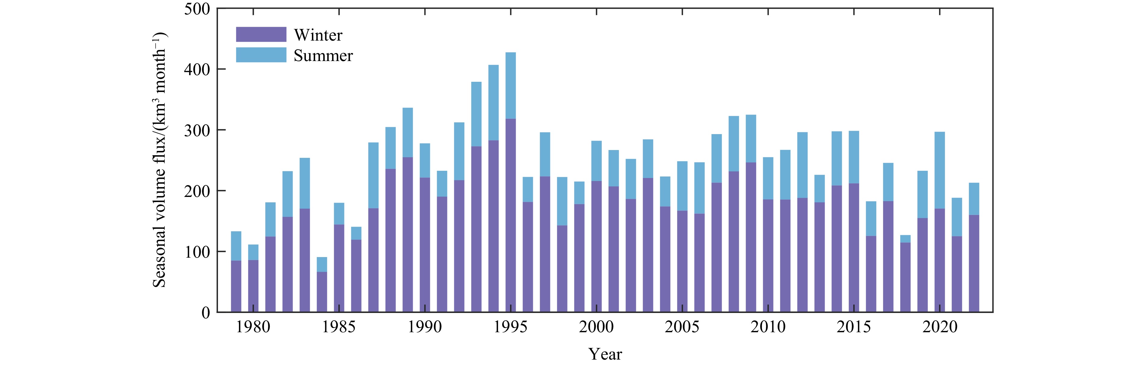
The sea ice volume flux through FS shows significant seasonal variations, with higher fluxes observed during winter (Fig. 4). In this study, winter is defined as the period from October to April, and summer refers to the months from May to September. On average, the flux in summer contributing 27.37% annual total while the winter accounting for 72.63%.
 Figure 4. Seasonal volume flux through FS during 1979–2022
3.2 Temporal and spatial variation of sea ice volume in the GS
As shown in Fig. 5, the sea ice volume in the GS from 1979 to 2022 exhibited no significant trend. However, a notable downward trend emerged during the period of 2001–2022, which was characterized by a decline rate of −5.36 km3/yr. Throughout the entire period of 1979–2022, all the months, except June (downward trend but do not pass the significance test), showed a significant downward trend. Notably, the winter months experienced a highly pronounced and rapid decrease, with January and March exhibiting a decreasing rate of −4.19 km3/yr and −4.46 km3/yr, respectively. Whether on an annual or on a monthly scale, the sea ice volume in the GS declined rapidly during the second period. Some studies demonstrated that the SIT has more influence on the sea ice volume compared with other factors, particularly during winter, when it can account for over 80% of the variability (Li, 2021). Thus, the accelerated decrease during the period of 2001–2022 indicates that the sea ice in the GS has been undergoing rapid thinning since the beginning of the 21st century (Liu et al., 2020; Li, 2021).
 Figure 5. Annual sea ice volume in the GS (a), monthly sea ice volume in the GS in 1979–2022 ((b)–(m)), representing January to December. The solid trend lines denote passing significant test.
The changes in the sea ice volume in the GS are influenced by a combination of advection and local factors. The sea ice volume in the GS exhibits a decreasing trend, whereas no significant trend can be seen in the sea ice volume flux, which indicates that sea ice melting is increasing rapidly. When the sea ice flux replenishment fails to offset the sea ice melting, it may reduce the sea ice volume, which shows that the local processes on sea ice melting in the GS is strengthening.
As depicted in Fig. 6a, the distribution of the effective SIT in the GS exhibits a V-shaped pattern from north to south, with thick sea ice concentrated primarily in the northern region. During the period of 1979–2000, the sea ice was distributed extensively, and the effective SIT ranged from (1.00 m ± 0.50 m; Fig. 6b). However, compared with the first period, the sea ice extent decreased noticeably and shifted northward during the period of 2001–2022 (Fig. 6c). In addition, the effective SIT decreased significantly within the range of (0.05 m ± 0.03 m).
 Figure 6. Spatial distribution of effective SIT in the GS during 1979–2022 (a), 1979–2000 (b), and 2001–2022 (c).
During the period of 1979–2022, the rate of change in the effective SIT in the GS showed a decreasing trend, with a T-distribution (Fig. 7a). During the period of 1979–2000, the areas that exhibited thickness changed rapidly, primarily around 12 °W, within the range of (−0.01± 0.02) m/yr (Fig. 7b). The spatial distribution of the decreasing SIT trend during the period of 2000–2022 was also a T-distribution, ranging from (−0.02±0.04) m/yr (Fig. 7c).
 Figure 7. Spatial distribution of effective SIT change rate in the GS during 1979–2022 (a), 1979–2000 (b), and 2001–2022 (c).
3.3 Temporal and spatial variation in SAT and SST
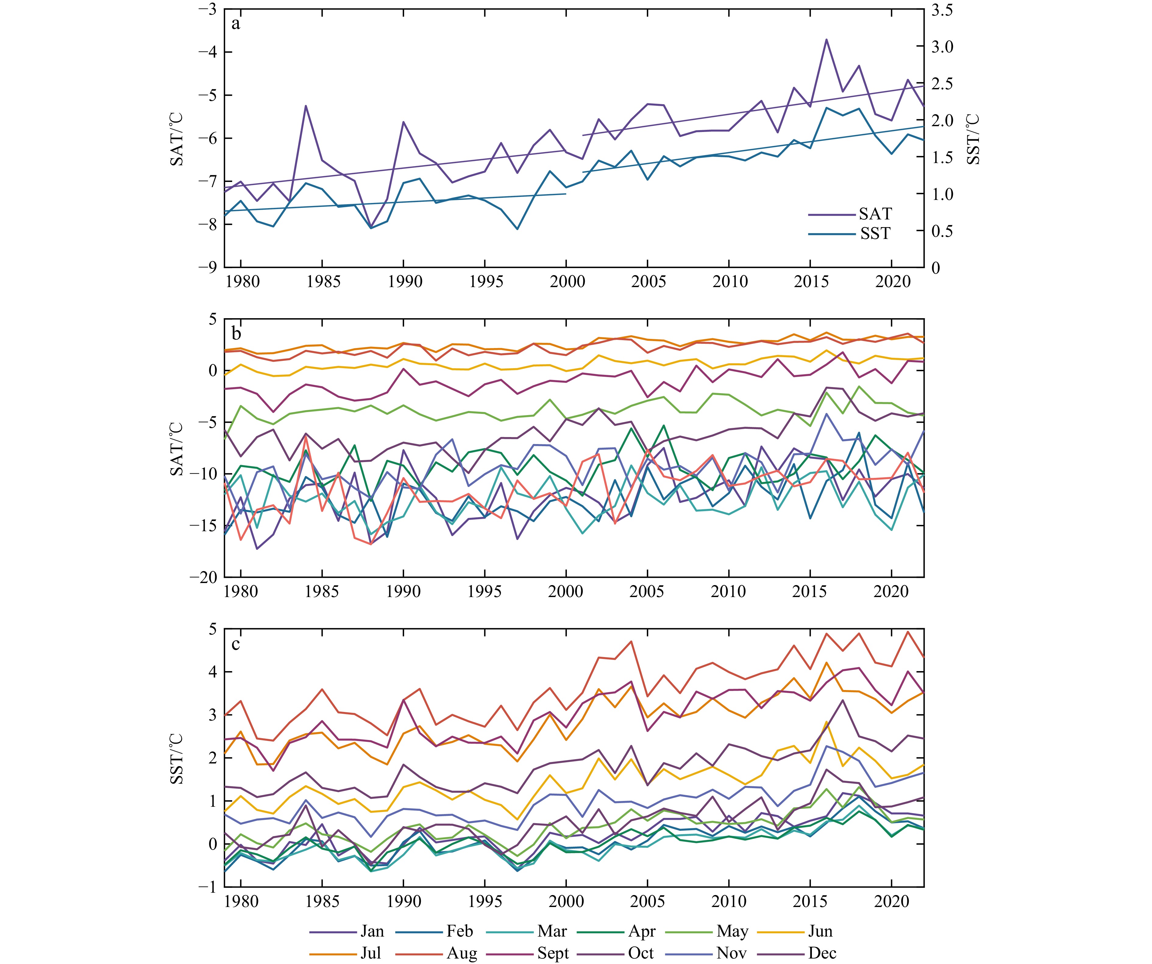
During the period of 1979–2000, the SST and SAT exhibited an upward trend but do not pass the significance test. However, during the period of 2001–2022, the SST and the SAT showed a significant increase. The years with extreme values generally coincided with one another, with maximum values in 1984, 1990, and 2016 and minimum values in 1988 and 1997. The warming of the SST and the SAT at the beginning of the 21st century accelerated sea ice melting, which corresponds to the accelerated decline of sea ice observed in the second period.
As depicted in Fig. 8b and Fig. 8c, the SAT reached the highest value in July and the lowest value in February, whereas the SST generally reached the highest value in August and the lowest value in March. During the months with extreme temperatures, a one-month lag can be seen in the SST compared with the SAT. This lag can be attributed to the larger specific heat capacity of the ocean compared with that of the atmosphere (Li, 2021). The ocean absorbs the same amount of energy but undergoes a relatively small temperature change. In addition, temperature changes from water mixing in the ocean require a long period of time. The slow heat transfer process caused by ocean currents can contribute to the delayed response of the SST to external changes. The combined factors can result in a one-month lag in the SST compared with the SAT.
 Figure 8. Annual SAT and SST (a), monthly SAT (b), monthly SST (c) during 1979–2022.
As depicted in Fig. 9a, the spatial changes in the SST from 1979 to 2000 show a decreasing trend in the northwest region and an increasing trend in the southeast region, with the most noticeable warming areas located along the coast of Svalbard and in the Denmark Strait. During the period of 1979–2000, the changes in the SST were relatively small, with a warming area located on the southern side of Svalbard and few cooling areas (Fig. 9b). However, the changes in the SST were highly pronounced during the period of 2001–2022 (Fig. 9c). The spatial distribution exhibits cooling in the northwest and warming in the southeast. Notably, the warming area shifted significantly northward in the second period compared with that in the first period, and the rate of warming demonstrated a significant increase.
 Figure 9. Spatial distribution of annual average SST/SAT change rates during 1979–2022 (a)/(d), 1979–2000 (b)/(e), and 2001–2022 (c)/(f).
The spatial distribution of the SAT changes appears to be highly consistent and smooth (Figs. 9a–c). During the different periods, a general warming trend can be observed in the northeast and southwest regions, whereas a cooling trend is evident in the northwest and southeast regions.
4. Discussion
4.1 Variations of sea ice volume flux through FS and sea ice volume in the GS
To facilitate the comprehensive comparison of the impact of ice advection from the north and local processes on sea ice changes, this study applies a sign convention to the volume variations attributed to local forcing. Specifically, in Fig. 10, the positive values indicate a reduction in the sea ice volume in the GS, whereas the negative values represent an increase in the volume.
 Figure 10. Sea ice volume variations in the GS for advection and local factors at annual (a), winter (b), and summer (c).
Sea ice volume variations influenced by advection and local forcing exhibit similar trends (Figs. 10a–c). During winter, the impact of ice advection from the north on sea ice volume variations is typically greater than that of local processes (Fig. 10b). Conversely, during summer, the local processes have a greater influence (Fig. 10c). However, throughout the different periods, the sea ice advection primarily replenishes the sea ice, whereas the local forcing predominantly melts the sea ice. The balance between sea ice volume export to the GS through FS and regional changes is strongly influenced by the sea ice transport and local processes. The volume of sea ice in the GS and sea ice flux are not strongly correlated, indicating that the sea ice variability in the GS can be greatly affected by the local processes (Selyuzhenok et al., 2020; Chatterjee et al., 2021).
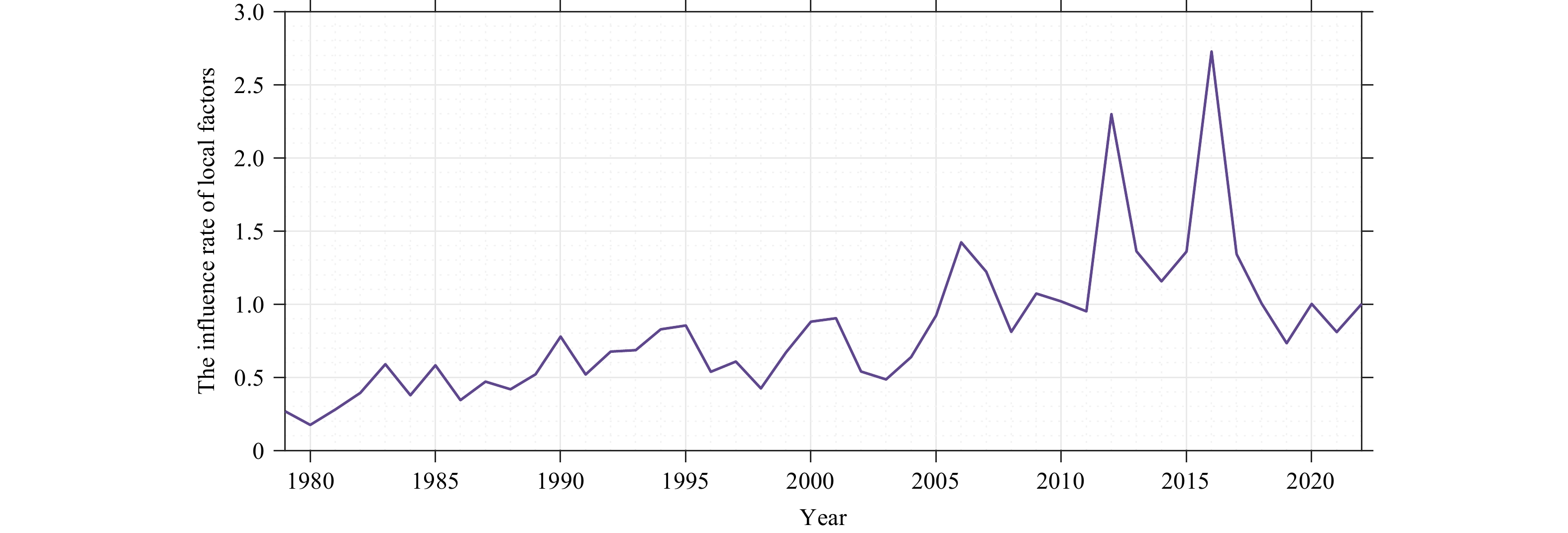
The variations in the sea ice volume induced by local factors are strongly linked with the local sea ice dynamics process and oceanic conditions (Campbell et al., 1987; Visbeck et al., 1995; Kern et al., 2010; Selyuzhenok et al., 2020; Chatterjee et al., 2021). The sea ice volume variations caused by ice advection from the north do not exhibit a significant trend, whereas the total sea ice volume in the GS displays a significant decreasing trend. Therefore, the influence of local factors may be masked by the overall decreasing trend of the sea ice volume. A highly accurate assessment of the impact of local factors on sea ice can be conducted by considering the rate of sea ice changes induced by local factors to the total sea ice volume. As shown in Fig. 11, before 2000, the influence of local factors on sea ice was relatively limited, with the rate remaining below 1. However, since the start of the 21st century, the rate has exhibited a sharp increase, reaching 2.30 in 2012 and 2.73 in 2016, which indicates the intensified local processes. The average annual Arctic sea ice volume in the GS in 2016 and 2012 is the minimum and sub-minimum (Fig. 5), respectively. The loss of sea ice led to more open water, along with anomaly high SAT and SST in 2012 and 2016 (Fig. 8), accelerating the melting of sea ice. As sea ice melts, the open water area in the GS will expand, which will lead to increased energy absorption by the ocean and further melting of the sea ice. On the other hand, low SLP over GS associated with stronger cyclonic Greenland Sea Gyre (GSG) and stronger Ekman drift, which will weaken the upper-ocean stratification and enhanced vertical mixing of anomalous warm Atlantic Water (AW) by reducing the freshwater in the GS. Under the weak stratification condition, the AW will warm the surface waters by enhanced vertical mixing and then further inhibiting new sea ice formation or melting the sea ice from bottom (Ivanova et al., 2012). The increased salinity caused by the vertical mixing further promotes a stronger GSG circulation and then reduce sea ice in the region, completing a positive feedback mechanism (Lauvset et al., 2018; Chatterjee et al., 2021).
 Figure 11. The annual influence rate of local factors in 1979–2022.
4.2 Changes in sea ice volume related to the SAT and SST
The sea ice volume in the GS exhibits a strong correlation with the SAT and the SST. The SAT and the SST demonstrate a significant increasing trend (Fig. 12) and have a negative correlation with the sea ice volume in the GS.
 Figure 12. The correlation between variability of sea ice volume due to local forcing in the GS and SAT and SST at different lag months.
As depicted in Fig. 12, the impact of the SAT on the sea ice volume exhibits a lag of approximately 2 to 3 months, and that of the SST exhibits a lag of 1 to 2 months. In terms of lag, the SAT exhibits the earliest change, thereby influencing the SST, which in turn indirectly affects the sea ice through the SST. The sea ice growth and melting can be determined by the heat exchange processes occurring within, on top, and at the bottom of the sea ice. Such processes are jointly controlled by the SAT and the SST. When the SST reaches the freezing point (−1.8°C), the density of the sea will increase, then decrease, and warm water from the Atlantic Ocean will rise to the surface and exchange heat with the surface air once again. Sea ice will not begin to melt until the warm water that rose to the surface reaches the freezing point (Li, 2021). In addition, sea ice exchanges heat with the environment as it grows and melts, which in turn can affect the changes in the SAT and in the SST.
The SST and SAT anomalies are analyzed using the EOF to obtain the spatial distribution and corresponding time series coefficients of their first two modes. The first mode of the SST captures the interdecadal scale changes, and when combined with the time series coefficients (Fig. 13b), it reveals two contrasting anomalies. Specifically, anomalously low SST can be observed during the period of 1979–2000, followed by anomalously high SST during the period of 2000–2022. The areas experiencing rapid warming are concentrated along the coast of Svalbard and on the eastern side of the Denmark Strait (Fig. 13a), which correspond to the areas of the Irminger current and the West Spitsbergen current. Conversely, the slow warming observed along the eastern coast of GS can be attributed to the presence of the East Greenland current, which transports cold water from the Arctic. The first mode of the SAT exhibits characteristics similar to those of the SST (Fig. 13e), with anomalously low temperatures before 2000 and anomalously high temperatures after 2000. However, its interdecadal characteristics are less pronounced than those of the SST (Fig. 13f), because the SAT is more susceptible to climatic events, which may result in many frequent fluctuations.
 Figure 13. Spatial distribution modes and time series coefficients for the EOF analysis of SST (a)–(d) and SAT anomaly (e)–(h).
The second mode of the SST captures the interannual variability in the SST and reveals that the regions with high SST values and positive time coefficients align closely with the areas with a rapidly decreasing effective SIT (Fig. 7a). The regions form distinct stripes that extend southward from the northern part of the Svalbard Archipelago (Fig. 13c). The least squares fit analysis of the time coefficients of the second mode after 2000 (Fig. 13d) reveals a significant upward trend (0.04). This finding indicates that the warming pattern observed in the striped region occurred frequently after 2000, which corresponds to the rapid decline in the sea ice volume in the GS during the period. When combined with the time coefficients (Fig. 13h), it shows that the northwest region experienced anomalous warming during the period of 1979–2000, whereas the southeastern region experienced anomalous warming during the period of 2001–2022. The second mode of the SST exhibits a spatial distribution characterized by a seesaw pattern of opposite changes in the northwest and southeast regions (Fig. 11g), which has been more variable after 2000. The oceanic temperature may be responsible for the sea ice variation in the GS, which consistent with other study that show the sea ice volume loss in the GS are largely determined by the oceanic conditions (Selyuzhenok et al., 2020).
4.3 Effects of atmospheric circulation patterns
The AO index has a considerable influence on the volume flux. Numerous studies highlighted the impact of the AO on sea ice motion and emphasized its significant association with sea ice output from FS (Zhang et al., 2003, 2023; Kwok et al., 2013; Howell and Brady, 2019). During a positive AO, the sea surface pressure in the Arctic region decreases, which will weaken the Beaufort anticyclonic circulation. This weakening will enhance the cyclonic tendency of the sea ice movement, resulting in a westward shift of the transpolar drift centerline. Consequently, an increased amount of sea ice, particularly from the northern region of the Canadian Arctic Archipelago, will flow out through FS (Rigor et al., 2002). Conversely, during a negative AO, the intensification of the Beaufort anticyclone will facilitate the transport of sea ice from the western part of the Arctic Basin to the east through enhanced easterly anomalous winds. This process can suppress the export of sea ice (Rigor and Wallace, 2004). A significant correlation (0.47) can be observed between AO and the FS volume flux before 2000 (Fig. 14a). However, this relationship became insignificant (r = 0.10) after 2000 (Fig. 14b). The correlation analysis reveals a weakening relationship between the AO and sea ice output during winter. The reduction in sea ice thickness may be responsible for the decreased correlation, as it alters the dynamics of sea ice and making it less responsive to AO variations. The effect of NAO on sea ice output is similar to that of AO but less significant.
 Figure 14. Correlation between atmospheric circulation indices and sea ice volume flux through FS (a)–(c). * indicates passing the significance test (p<0.05).
DA is also an important driving force for the transport of Arctic sea ice to the North Atlantic. When DA is in positive phase (positive SLP anomaly in the Canadian Islands, negative anomaly in the Barents Sea), the meridional wind blows from the west to the east and enhances the Transpolar Drift, increasing Arctic sea ice output (Wu et al., 2006; Wang et al., 2009; Zhang et al., 2022). In terms of correlation (Fig. 14c), DA exerts greater effect on sea ice output than AO (NAO). The positive phases of DA consistently promote sea ice export during summer (r = 0.37) and winter (r = 0.43) in 1979–2022.
Since SST is closely correlated with the local sea ice in the GS (Section 4.2), we calculated the correlation between SST and AO/NAO/DA index. The results indicate that NAO has greater impact on SST (r = 0.26), while AO (r = 0.01) and DA (r = −0.13) are not significant. NAO is the leading mode of the pressure variability in the northern North Atlantic (Woollings et al., 2010; Moore and Renfrew, 2012; Foukal and Lozier, 2017; Selyuzhenok et al., 2020), and plays a crucial role in regulating ocean circulation in the NS. Specifically, during the positive phase of the NAO, the cyclonic atmospheric circulation over NS become stronger and results in the cyclonic oceanic circulation in NS intensifies (Schlichtholz and Houssais, 2011). This leads to weaker upper-ocean stratification and stronger vertical mixing of anomalous warm AW, increasing the temperature in the upper ocean (Section 4.1).
To investigate the influence of NAO on the ocean circulation, we calculated upper 300 m OHC over the GS. The reduction of sea ice in the GS are partially driven by the increasing of OHC. As illustrated in Fig. 15, OHC exhibits no significant trend in 1979–2000. After 2000, however, an increasing trend in OHC was highly pronounced coincides with the loss of sea ice in the GS. Compared to the period before 2000, the correlation between winter NAO and OHC increased from 0.08 to 0.40 during the period of 2001–2022 (Table 2), which indicated that the winter NAO has a greater influence on the oceanic systems after 2000. This finding is consistent with previous studies revealed that a stronger oceanic heat advection during the positive NAO (Walczowski, 2010; Raj et al., 2018). This suggests that the positive winter NAO may accelerate the melting of sea ice by increasing OHC. This is confirmed by Ivanova et al. (2012), who exhibited enhanced bottom melting in this region associated with positive NAO.
 Figure 15. Annual Upper 300 m OHC, summer NAO (May–September) and winter NAO (October–April) during 1979-2022. The purple solid trend line denotes passing significant test.Table 2. Correlations between summer/winter NAO and OHC.
1979–2022 1979–2000 2001–2022 Summer NAO and OHC −0.16 0.05 0.15 Winter NAO and OHC 0.17 0.08 0.40* Note: * indicates passing the significance test (p<0.05). | Show TableDownLoad:
CSV
5. Conclusions
In this study, we calculate the sea ice volume flux through FS and the sea ice volume in the GS from 1979 to 2022 using SID data from the NSIDC and effective SIT data from the PIOMAS. We discuss the trends in two periods, namely, before and after 2000. We investigate the changes in the sea ice driven by advection and local processes, as well as the influence of the SAT, SST, and atmospheric circulation on the sea ice in the GS. The main conclusions of our study are as follows:
(1) The sea ice volume flux through FS exhibited no significant trend from 1979 to 2022. The annual average volume flux was 136 km3, and the volume flux displayed obvious seasonality, with a considerably large output during winter. Specifically, the winter output accounts for 72.63% of the total volume flux during the season.
(2) The sea ice volume in the GS did not exhibit a significant trend during the period of 1979–2000. However, it showed a notable decreasing trend, with a rate of −5.36 km3/yr, during the period of 2001–2022, particularly during the winter months. The highest sea ice volume was observed in 1989, which reached 395 km3, whereas the lowest value was recorded in 2016, which was only 89 km3. The sea ice volume in the GS is experiencing a rapid decline, whereas the reduction for advection in the sea ice has yet to demonstrate any significant changes. This finding suggests that the increasing influence of local forcing in the GS.
(3) The impact of the SST on sea ice is more pronounced than that of the SAT. A three-month lag can be seen in the influence of the SAT on sea ice, and a two-month lag can be observed in the influence of the SST, and the correlation between the SST and sea ice (r = −0.56) is slightly higher than that between the SAT and sea ice (r = −0.52). In addition, the second mode obtained from the EOF analysis of the SST aligns closely with the region of rapid changes in the effective SIT, which suggests that the SST plays an important role in the decline of sea ice.
(4) The AO index exhibited a positive correlation of 0.47 with the volume flux of the sea ice through FS in the period of 1979–2000. However, this correlation became insignificant after 2000 (r = 0.10), and DA exerted a greater effect on sea ice output than AO in this period. NAO has an important impact on the sea ice flux and it intensified the OHC in the GS in 2001−2022 (r = 0.40), which significantly effects the variability of sea ice in this region.
The effects of the atmosphere and the ocean on sea ice should also be assessed quantitatively, because merely considering the temperature is insufficient. Considering the multifaceted impact is essential to gain a comprehensive understanding of the complex processes that occur in the atmosphere and in the ocean and their influence on sea ice, as well as the feedback of sea ice to the atmosphere and the ocean, which can help us accurately predict Arctic sea ice changes and understand Arctic climate change. In the future, the effect of diverse factors on the sea ice volume output and the sea ice volume variations should be analyzed to determine the key factors and enhance understanding of the influence of different driving factors. Further investigation is needed to understand the mechanisms of how NAO and other atmospheric circulation patterns affect sea ice through oceanic processes.
Acknowlegements
The authors sincerely acknowledge the National Snow and Ice Data Center, the Pan-Arctic Ice Ocean Modeling and Assimilation System, the National Oceanic and Atmospheric Administration, and the European Centre for Medium-Range Weather Forecasts for providing the data. We are also deeply grateful to the Bi and Wang teams for their generous contribution of data for DA.
-
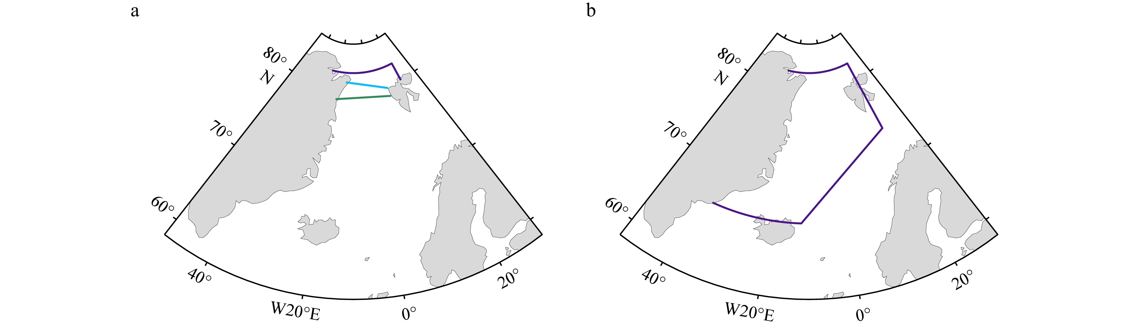
Figure 1. The flux gate (a) and the research area (b). The Purple line denotes flux gate of this paper and Ricker et al. (2018), while green line is Kwok et al. (2004) and blue line is Li (2021).

Figure 2. Comparison of sea ice volume fluxes with other studies (Kwok et al. (2004), Ricker et al. (2018); Li (2021)). The line is the monthly volume flux, the circle is the monthly volume flux in winter.

Figure 3. Annual volume flux through FS (a), monthly volume through FS in 1979–2022 ((b)–(m)), representing January to December. The solid trend lines denote passing significant test.

Figure 5. Annual sea ice volume in the GS (a), monthly sea ice volume in the GS in 1979–2022 ((b)–(m)), representing January to December. The solid trend lines denote passing significant test.

Figure 6. Spatial distribution of effective SIT in the GS during 1979–2022 (a), 1979–2000 (b), and 2001–2022 (c).

Figure 7. Spatial distribution of effective SIT change rate in the GS during 1979–2022 (a), 1979–2000 (b), and 2001–2022 (c).
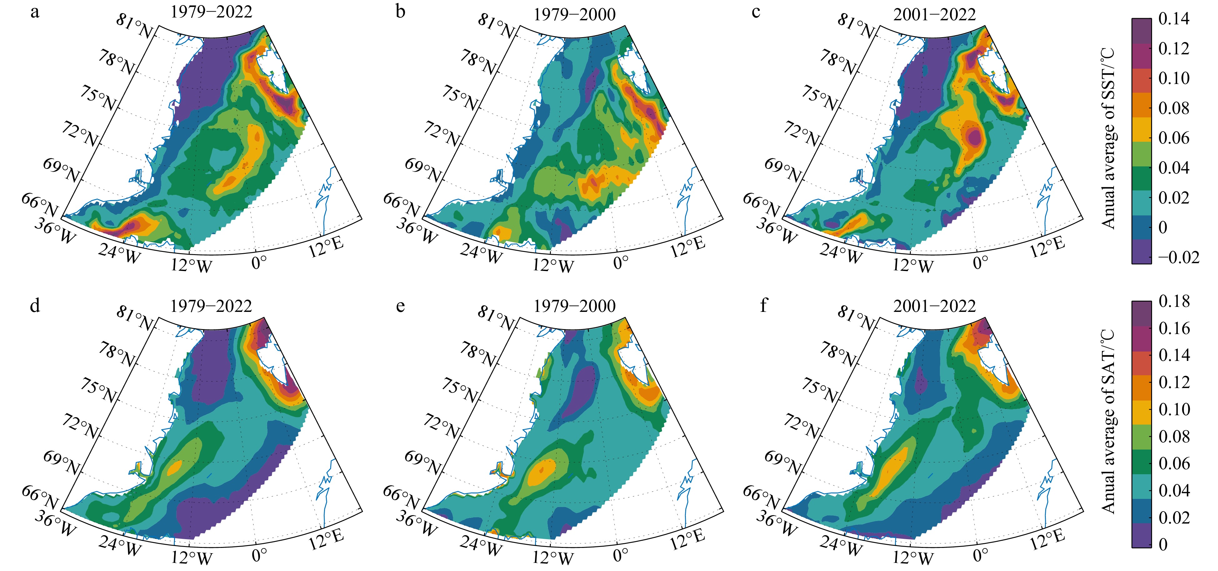
Figure 9. Spatial distribution of annual average SST/SAT change rates during 1979–2022 (a)/(d), 1979–2000 (b)/(e), and 2001–2022 (c)/(f).
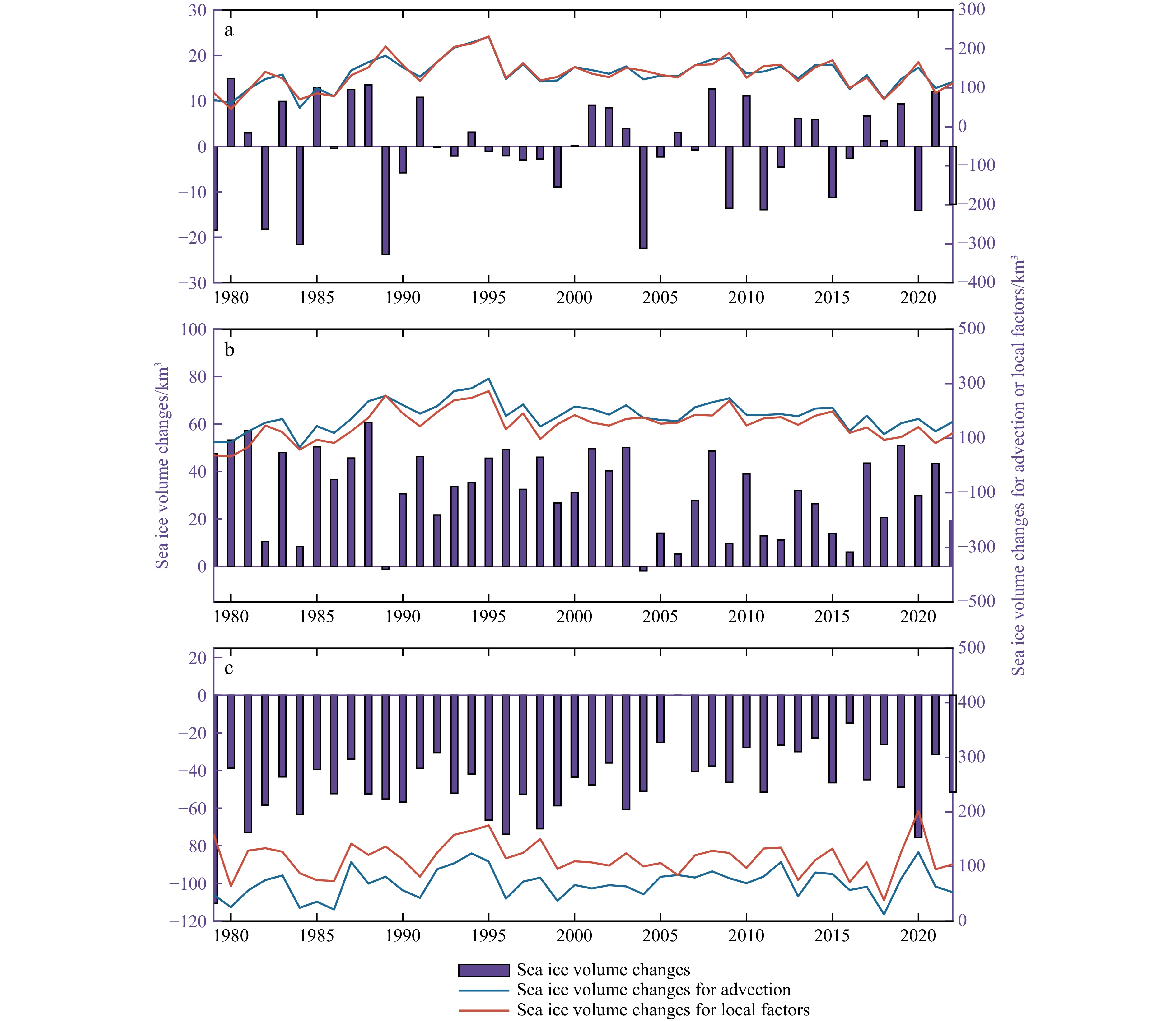
Figure 10. Sea ice volume variations in the GS for advection and local factors at annual (a), winter (b), and summer (c).
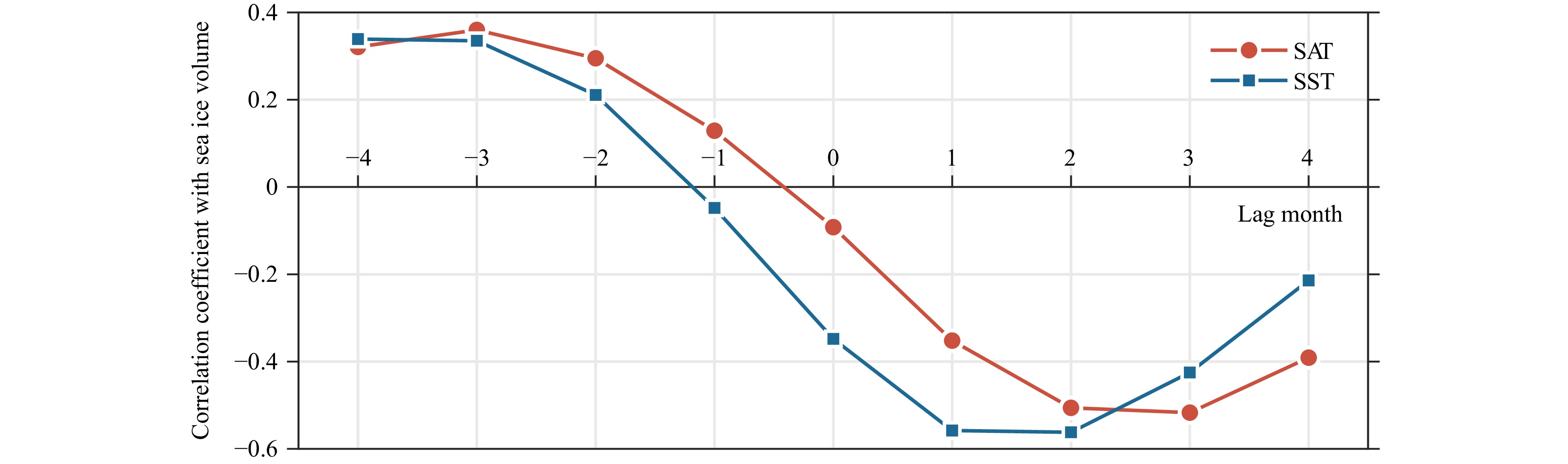
Figure 12. The correlation between variability of sea ice volume due to local forcing in the GS and SAT and SST at different lag months.

Figure 13. Spatial distribution modes and time series coefficients for the EOF analysis of SST (a)–(d) and SAT anomaly (e)–(h).

Figure 14. Correlation between atmospheric circulation indices and sea ice volume flux through FS (a)–(c). * indicates passing the significance test (p<0.05).

Figure 15. Annual Upper 300 m OHC, summer NAO (May–September) and winter NAO (October–April) during 1979-2022. The purple solid trend line denotes passing significant test.
Table 1. Comparison of volume flux with other studies
This paper Li (2021) Kwok et al. (2004) Ricker et al. (2018) SIC -- NSIDC ULS moorings OSI SAF SIT PIOMAS Envisat/NSIDC/IceBridge ULS moorings AWI CryoSat-2 SID NSIDC NSIDC Kwok and Rothrock (1999) OSI SAF Cor. -- 0.78* 0.69* 0.88* Note: * indicates passing the significance test (p<0.05).  下载: 导出CSV
Table 2. Correlations between summer/winter NAO and OHC.
1979–2022 1979–2000 2001–2022 Summer NAO and OHC −0.16 0.05 0.15 Winter NAO and OHC 0.17 0.08 0.40* Note: * indicates passing the significance test (p<0.05).
下载: 导出CSV
-
Arfeuille G, Mysak L A, Tremblay L B. 2000. Simulation of the interannual variability of the wind-driven Arctic sea-ice cover during 1958-1998. Climate Dynamics, 16(2–3): 107–121, doi: 10.1007/PL00013732 Bi Haibo, Wang Yunhe, Zhang Wenfeng, et al. 2018. Recent satellite-derived sea ice volume flux through the Fram Strait: 2011–2015. Acta Oceanologica Sinica, 37: 107–115. Bi Haibo, Yang Qinghua, Liang Yu, et al. 2018. A review of Arctic sea ice export. Marine Sciences (in Chinese), 42(10): 110–124 Blunden J, Arndt D S. 2017. State of the climate in 2016. Bulletin of the American Meteorological Society, 98(8): Si–S280, doi: 10.1175/2017BAMSStateoftheClimate.1 Brakstad A, Våge K, Håvik L, et al. 2019. Water mass transformation in the Greenland Sea during the Period 1986-2016. Journal of Physical Oceanography, 49(1): 121–140, doi: 10.1175/JPO-D-17-0273.1 Campbell W J, Gloersen P, Josberger E G, et al. 1987. Variations of mesoscale and large-scale sea ice morphology in the 1984 Marginal Ice Zone Experiment as observed by microwave remote sensing. Journal of Geophysical Research: Oceans, 92(C7): 6805–6824, doi: 10.1029/JC092iC07p06805 Chatterjee S, Raj R P, Bertino L, et al. 2021. Combined influence of oceanic and atmospheric circulations on Greenland sea ice concentration. The Cryosphere, 15(3): 1307–1319, doi: 10.5194/tc-15-1307-2021 Foukal N P, Lozier M S. 2017. Assessing variability in the size and strength of the North Atlantic subpolar gyre. Journal of Geophysical Research: Oceans, 122(8): 6295–6308, doi: 10.1002/2017JC012798 Howell S E L, Brady M. 2019. The dynamic response of sea ice to warming in the Canadian arctic archipelago. Geophysical Research Letters, 46(22): 13119–13125, doi: 10.1029/2019GL085116 Howell S E L, Wohlleben T, Dabboor M, et al. 2013. Recent changes in the exchange of sea ice between the Arctic Ocean and the Canadian arctic archipelago. Journal of Geophysical Research: Oceans, 118(7): 3595–3607, doi: 10.1002/jgrc.20265 Ivanova D P, McClean J L, Hunke E C. 2012. Interaction of ocean temperature advection, surface heat fluxes and sea ice in the marginal ice zone during the North Atlantic Oscillation in the 1990s: a modeling study. Journal of Geophysical Research: Oceans, 117(C2): C02031 Kern S, Kaleschke L, Spreen G. 2010. Climatology of the Nordic (Irminger, Greenland, Barents, Kara and white/Pechora) seas ice cover based on 85 GHz satellite microwave radiometry: 1992-2008. Tellus A, 62(4): 411–434, doi: 10.1111/j.1600-0870.2010.00457.x Kwok R. 2009. Outflow of Arctic Ocean sea ice into the Greenland and Barents seas: 1979-2007. Journal of Climate, 22(9): 2438–2457, doi: 10.1175/2008JCLI2819.1 Kwok R, Cunningham G F, Pang Shuxian. 2004. Fram Strait sea ice outflow. Journal of Geophysical Research: Oceans, 109(C1): C01009 Kwok R, Rothrock D A. 1999. Variability of Fram Strait ice flux and North Atlantic Oscillation. Journal of Geophysical Research: Oceans, 104(C3): 5177–5189, doi: 10.1029/1998JC900103 Kwok R, Spreen G, Pang Shuxian. 2013. Arctic sea ice circulation and drift speed: decadal trends and ocean currents. Journal of Geophysical Research: Oceans, 118(5): 2408–2425, doi: 10.1002/jgrc.20191 Landrum L, Holland M M. 2020. Extremes become routine in an emerging new Arctic. Nature Climate Change, 10(12): 1108–1115, doi: 10.1038/s41558-020-0892-z Lauvset S K, Brakstad A, Våge K, et al. 2018. Continued warming, salinification and oxygenation of the Greenland Sea gyre. Tellus A, 70(1): 1476434, doi: 10.1080/16000870.2018.1476434 Li Mengmeng. 2021. Analysis of Arctic sea ice volume change and its influencing factors based on the fusion of remote sensing and model data (in Chinese)[dissertation]. Nanjing: Nanjing University Lindsay R W, Schweiger A. 2015. Arctic sea ice thickness loss determined using subsurface, aircraft, and satellite observations. The Cryosphere, 9(1): 269–283, doi: 10.5194/tc-9-269-2015 Lindsay R W, Zhang Jinlun. 2005. The thinning of Arctic sea ice, 1988-2003: have we passed a tipping point? Journal of Climate, 18(22): 4879–4894 Lindsay R W, Zhang Jinlun, Schweiger A, et al. 2009. Arctic sea ice retreat in 2007 follows thinning trend. Journal of Climate, 22(1): 165–176, doi: 10.1175/2008JCLI2521.1 Liu Yinghui, Key J R, Wang Xuanji, et al. 2020. Multidecadal Arctic sea ice thickness and volume derived from ice age. The Cryosphere, 14(4): 1325–1345, doi: 10.5194/tc-14-1325-2020 Maslanik J, Stroeve J, Fowler C, et al. 2011. Distribution and trends in Arctic sea ice age through spring 2011. Geophysical Research Letters, 38(13): L13502 Moore G W K, Renfrew I A. 2012. Cold European winters: interplay between the NAO and the East Atlantic mode. Atmospheric Science Letters, 13(1): 1–8, doi: 10.1002/asl.356 Parkinson C L, Comiso J C. 2013. On the 2012 record low Arctic sea ice cover: combined impact of preconditioning and an August storm. Geophysical Research Letters, 40(7): 1356–1361, doi: 10.1002/grl.50349 Raj R P, Nilsen J E Ø, Johannessen J A, et al. 2018. Quantifying Atlantic Water transport to the Nordic Seas by remote sensing. Remote Sensing of Environment, 216: 758–769, doi: 10.1016/j.rse.2018.04.055 Rampal P, Weiss J, Marsan D. 2009. Positive trend in the mean speed and deformation rate of Arctic sea ice, 1979-2007. Journal of Geophysical Research: Oceans, 114(C5): C05013 Ricker R, Girard-Ardhuin F, Krumpen T, et al. 2018. Satellite-derived sea ice export and its impact on Arctic ice mass balance. The Cryosphere, 12(9): 3017–3032, doi: 10.5194/tc-12-3017-2018 Rigor I G, Wallace J M, 2004. Variations in the age of Arctic sea-ice and summer sea-ice extent. Geophysical Research Letters, 31(9): 111–142 Rigor I G, Wallace J M, Colony R L. 2002. Response of sea ice to the Arctic oscillation. Journal of Climate, 15(18): 2648–2663, doi: 10.1175/1520-0442(2002)015<2648:ROSITT>2.0.CO;2 Schlichtholz P, Houssais M N. 2011. Forcing of oceanic heat anomalies by air-sea interactions in the Nordic Seas area. Journal of Geophysical Research: Oceans, 116(C1): C01006 Schweiger A, Lindsay R, Zhang Jinlun, et al. 2011. Uncertainty in modeled Arctic sea ice volume. Journal of Geophysical Research: Oceans, 116(C8): C00D06 Selyuzhenok V, Bashmachnikov I, Ricker R, et al. 2020. Sea ice volume variability and water temperature in the Greenland Sea. The Cryosphere, 14(2): 477–495, doi: 10.5194/tc-14-477-2020 Smedsrud L H, Halvorsen M H, Stroeve J C, et al. 2017. Fram Strait sea ice export variability and September Arctic sea ice extent over the last 80 years. The Cryosphere, 11(1): 65–79, doi: 10.5194/tc-11-65-2017 Spreen G, de Steur L, Divine D, et al. 2020. Arctic sea ice volume export through Fram Strait from 1992 to 2014. Journal of Geophysical Research: Oceans, 125(6): e2019JC016039, doi: 10.1029/2019JC016039 Spreen G, Kern S, Stammer D, et al. 2009. Fram Strait sea ice volume export estimated between 2003 and 2008 from satellite data. Geophysical Research Letters, 36(19): L19502 Spreen G, Kwok R, Menemenlis D. 2011. Trends in Arctic sea ice drift and role of wind forcing: 1992-2009. Geophysical Research Letters, 38(19): L19501 Stroeve J C, Serreze M C, Fetterer F, et al. 2005. Tracking the Arctic’s shrinking ice cover: another extreme September minimum in 2004. Geophysical Research Letters, 32(4): L04501 Sumata H, de Steur L, Gerland S, et al. 2022. Unprecedented decline of Arctic sea ice outflow in 2018. Nature Communications, 13(1): 1747, doi: 10.1038/s41467-022-29470-7 Visbeck M, Fischer J, Schott F. 1995. Preconditioning the Greenland Sea for deep convection: ice formation and ice drift. Journal of Geophysical Research: Oceans, 100(C9): 18489–18502, doi: 10.1029/95JC01611 Walczowski W. 2010. Atlantic Water in the Nordic Seas–properties, variability, climatic significance. Oceanologia, 52(2): 325–327 Wang Kun, Bi Haibo, Huang Jue. 2022. Ice output of the Fram Strait sea in the past four decades based on remote sensing data. Marine Sciences (in Chinese), 46(4): 44–54 Wang Yunhe, Bi Haibo, Huang Haijun, et al. 2019. Satellite-observed trends in the Arctic sea ice concentration for the period 1979–2016. Journal of Oceanology and Limnology, 37: 18–37 Wang Jia, Zhang Jinlun, Watanabe E, et al. 2009. Is the Dipole Anomaly a major driver to record lows in Arctic summer sea ice extent? Geophysical Research Letters, 36(5): L05706 Woollings T, Hannachi A, Hoskins B. 2010. Variability of the North Atlantic eddy-driven jet stream. Quarterly Journal of the Royal Meteorological Society, 136(649): 856–868, doi: 10.1002/qj.625 Wu Bingyi, Wang Jia, Walsh J E. 2006. Dipole anomaly in the winter Arctic atmosphere and its association with sea ice motion. Journal of Climate, 19(2): 210–225, doi: 10.1175/JCLI3619.1 Zhang Xiangdong, Ikeda M, Walsh J E. 2003. Arctic sea ice and freshwater changes driven by the atmospheric leading mode in a coupled sea ice–ocean model. Journal of Climate, 16(13): 2159–2177, doi: 10.1175/2758.1 Zhang Fanyi, Lei Ruibo, Zhai Mengxi, et al. 2023. The impacts of anomalies in atmospheric circulations on Arctic sea ice outflow and sea ice conditions in the Barents and Greenland seas: case study in 2020. The Cryosphere, 17(11): 4609–4628, doi: 10.5194/tc-17-4609-2023 Zhang Fanyi, Pang Xiaoping, Lei Ruibo, et al. 2022. Arctic sea ice motion change and response to atmospheric forcing between 1979 and 2019. International Journal of Climatology, 42(3): 1854–1876, doi: 10.1002/joc.7340 Zhang Jinlun, Rothrock D A. 2003. Modeling global sea ice with a thickness and enthalpy distribution model in generalized curvilinear coordinates. Monthly Weather Review, 131(5): 845–861, doi: 10.1175/1520-0493(2003)131<0845:MGSIWA>2.0.CO;2 -

 DownLoad:


 点击查看大图
计量
- 文章访问数: 62
- HTML全文浏览量: 17
- 被引次数: 0