Figure  1.  Air-sea flux observation platforms. Symbol‘★’is the observation platform of Juehua Island, and‘▲’is the Yantai National Satellite Ocean Calibration Platform.

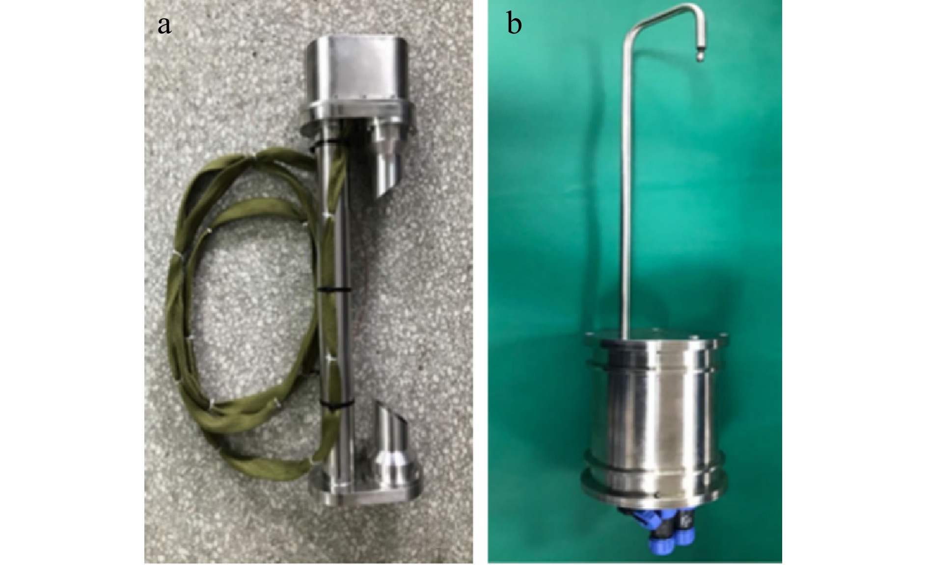
Figure  2.  High-frequency 100 Hz pulsating gas analyzer. (a) CO₂ gas analyzer; (b) H₂O gas analyzer.

Figure  3.  In situ observation experiments. (a) and (b) are the Yantai National Satellite Ocean Calibration Platform and the island observation platform at Juehua Island, Liaoning Province, respectively; (c) and (d) are the instrumentation of platforms (a) and (b), respectively.

Figure  4.  Raw data preprocessing and air-sea flux calculation flow chart. The dashed boxes represent steps that are not included in the main air-sea flux calculation process and are discussed separately in this article.

Figure  5.  Delay times. Delay time of ultrasonic anemometer with high-frequency CO₂ pulsometer (a) and with high-frequency water vapor pulsometer (b).

Figure  6.  Three-dimensional wind speed correction. (a) Before correction; (b) after correction. In the Fig., “○” is the average of 5 min wind speed samples from the offshore platform and the solid line is the vertical distance between “○” and the u-v plane.

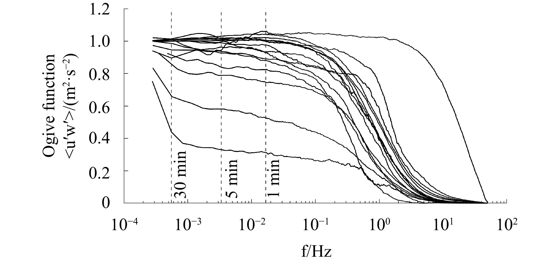
Figure  7.  Ogive curves of downwind and vertical wind speeds plotted for 16 randomly selected days from our July 2021 offshore platform observations, and randomly selecting 1 hour data each day. Each Ogive Curve corresponds to one hour of data from one of the days. $ z/L= 0 $.

Figure  8.  Water vapor flux WPL correction (July 10, 2021). Black lines indicate uncorrected air-sea fluxes; solid gray lines indicate corrected results; red dashed lines indicate the difference between pre-correction minus correction, and “//” indicates truncated invalid data.

Figure  9.  Wind speed power spectra. (a), (b), (c) and (d), (e), (f) are the power spectra of offshore platforms and island of $ u $, $ v $, and $ w $, respectively; solid gray lines indicate measured data, “○” indicates averaged data, and dashed lines indicate “–2/3” slopes.

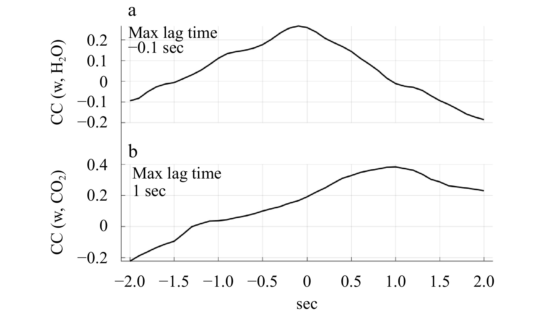
Figure  10.  Co-spectral analysis. (a), (b) are co-spectra of $ w $ with H₂O and CO₂, respectively. The solid gray line indicates co-spectra of $ w $ with H₂O (Fig. 10a) and CO₂ (Fig. 10b) respectively. And “●” indicates averaged co-spectra data, the dashed line indicates the “–4/3” slope; the solid black line indicates the Kaimal et al. (1972) is suitable for atmospheric stabilization.

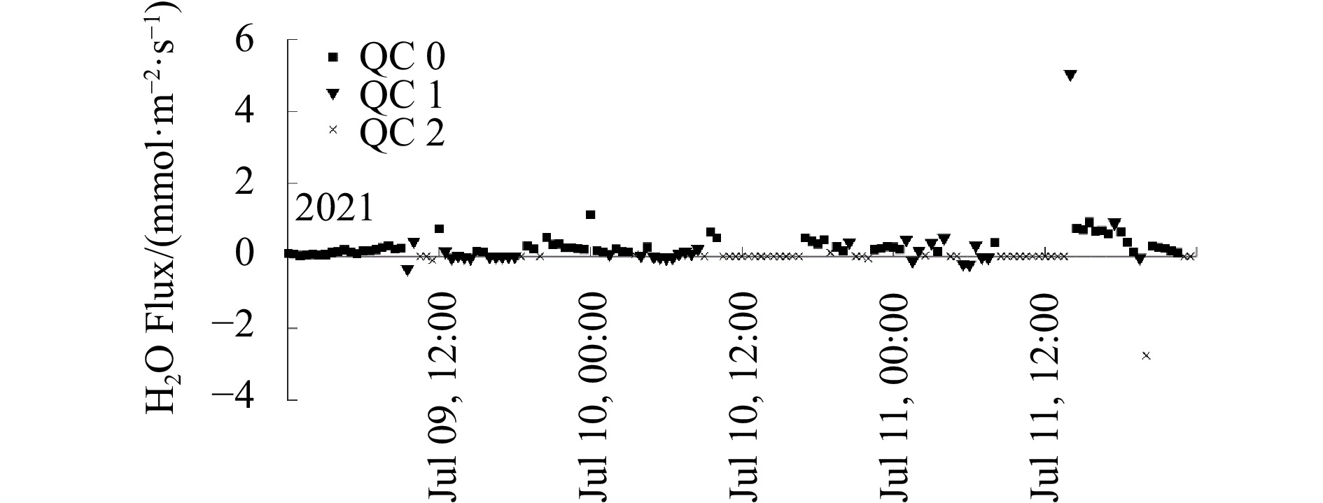
Figure  11.  Overall turbulence data quality for island water vapor flux observations. “■” denotes high quality data; “▼” denotes moderate quality data; “×” denotes invalid data.

Figure  12.  Air-sea flux observations from offshore platforms. (a) is the water vapor flux and (b) is the CO₂ flux. “▼” denotes 100 Hz frequency; “●” denotes 20 Hz frequency; dashed line denotes zero air-sea flux.

Figure  13.  Comparison of observed air-sea fluxes at different frequencies over the island. (a) Difference between 100 Hz and 20 Hz air-sea fluxes; (b), (c), and (d) are partial zoomed-in plots showing island air-sea flux observations on July 9, 10, and 11, 2021, respectively. The “//” denotes the axes of the truncated, partially invalid data, “▼” denotes 100 Hz, and “●” denotes 20 Hz.

Figure  14.  Water vapor and CO₂ concentrations over time; (a) and (b) are water vapor versus time for offshore platform and island data, respectively. The inner image of (a) is its local zoom; (c) is the CO₂ variation with time. The red solid line indicates 100 Hz observations and the black solid line indicates 20 Hz observations.

Figure  15.  Island and nearshore air-sea fluxes vary with wind speed; red dots indicate 100 Hz observed air-sea fluxes, black squares indicate 20 Hz observed air-sea fluxes; error bars indicate 95% confidence intervals.

Figure  16.  Trends and confidence analyses of air-sea CO₂ and water vapor fluxes; red dots indicate 100 Hz air-sea flux data, blue dots indicate 20 Hz air-sea flux data; red and blue lines indicate fitted curves; and shaded areas indicate 95% confidence limits.