

Figure
1.
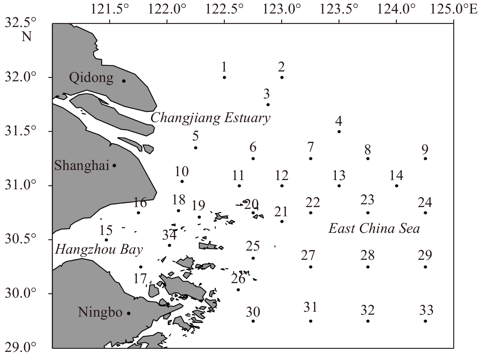
Study area and original sampling stations in 2007.
| Citation: | Chunyang Sun, Yingbin Wang. Impacts of the sampling design on the abundance index estimation of Portunus trituberculatus using bottom trawl[J]. Acta Oceanologica Sinica, 2020, 39(6): 48-57. doi: 10.1007/s13131-020-1607-z

|
Fisheries survey data are the basis of stock assessment and management (Jardim and Ribeiro, 2007). The assessment of total allowable catch (TAC), for example, must rely on the survey data. Therefore, it is necessary to obtain reliable survey data. The traditional survey method that is usually used to estimate abundance is sweep area method using otter trawls. Different designing principles and numbers of station affect the survey results (Stein and Ettema, 2003). Another impact factor is the target species, since different species, such as fish, cephalopod, crustacean, etc., have different reaction characteristics to the fishing gears and different swimming abilities, which will result in different vulnerabilities or escape rates (Yu, 2011).
Portunus trituberculatus is one of the important coastal economy species in China (Song et al., 2006). The total catch of P. trituberculatus in China exceeded 5×10⁵ t in 2016 (Fisheries and Fisheries Administration of the Ministry of Agriculture, 2017). Zhejiang Province, whose catch of P. trituberculatus account for about 35% of that in China, is the most high-yield province of P. trituberculatus. The catch of P. trituberculatus in Zhejiang Province increased about 30% during the past 10 years. In 2017, the Ministry of Agriculture (MOA) chose the northern Zhejiang fishing ground as a pilot area to carry out the catch quota management (CQM) of P. trituberculatus (Anonymous, 2018). CQM is currently a kind of advanced measure in fishery management. On the basis of scientific monitoring and assessment of fishery resources, a total allowable catch (TAC) of target species in a certain period of time will be determined, and then allocated (Huang and Huang, 2002). Scientific sampling design is the key point to improve the estimate quality of TAC, because it can obtain information about the target population such as resource abundance and distribution at a certain spatial-temporal scale (Jardim and Ribeiro, 2007). Additionally, the limitation of funds and complex marine geological conditions are frequently encountered problems in fishery surveys. Therefore, optimal sampling design is necessary, since it can save cost while ensuring the full use of data and maximize the investigation benefit (Simmonds and Fryer, 1996; Liu et al., 2009).
Fixed-station sampling is the most common method used in the survey of fishery resources in China. This method can be used to compare the dynamic changes of resources in different years by surveying resources at the fixed stations (Zhao et al., 2014; Wang et al., 2018). Simple random sampling is the most basic sampling method, which is the basis of other sampling methods, and is often used as the standard to compare with other sampling methods (Jin et al., 2008; Liu, 2012). Stratified random sampling is supported by the theory of classical statistics (Cochran, 1977; Manly et al., 2002; Miller et al., 2007), which is widely used in scientific investigation of fishery resources because it can make selected samples more representative, improve the estimation accuracy of parameters, and save the investigation cost as well (Smith and Gavaris, 1993; Gou, 2005; Xu et al., 2015). In the current study, we assessed four different sampling designs, including fixed-station sampling design (FS), simple random sampling design (SR), stratified fixed-station sampling design (SFS) and stratified random sampling design (SRS).
The studies about sampling designs were carried out as early as the 1980s. Gavaris and Smith (1987) and Smith and Gavaris (1993) conducted studies of sampling design on bottom trawl fisheries for the comparison of stratified random sampling and simple random sampling. Yuan et al. (2009) and Liu et al. (2009) are early researchers in this field in China (Liu et al., 2009; Yuan et al., 2009). In recent years, many scholars have studied the comparison and application of different sampling designs, as well as various factors affecting sampling precision (Cabral and Murta, 2004; Overholtz et al., 2006; Smith, 2006), the research objects (benthos, crustaceans, fish, etc.) have also been broadened (Skibo et al., 2008). With the development of computer technology, simulation analysis is becoming more and more popular in fishery resources surveys (Li et al., 2008; Yu et al., 2012; Wang and Jiao, 2015; Xu et al., 2015). However, there are neither studies about the sampling design for Portunus trituberculatus nor the reports about the algorithms for the survey by bottom trawl. Therefore, the goals of this study are to: (1) establish an algorithm based on probability of sweep area method; (2) compare the performances of different sampling designs in the study area; (3) compare the effectiveness of different number of stations when estimating the abundance of Portunus trituberculatus.
The study area in the current study is the Changjiang River Estuary-Hangzhou Bay and the adjacent area. Fishery resources are abundant in this sea area, and it is traditional fishing ground for fishermen in Zhejiang, Jiangsu, Fujian and Shanghai as well as Taiwan Province (Department of Fisheries, Ministry of Agriculture, Animal Husbandry and Fisheries, 1987; Zheng, 2003). The pilot water for the CMQ of the P. trituberculatus is right in this area (Fig. 1).
The distribution and density data of P. trituberculatu obtained from the bottom trawl survey in the Changjiang River Estuary-Hangzhou Bay and its adjacent waters (29°–32°N, 120°–125°E) in 2007 were used to simulate the “true” situation. The survey was carried out quarterly (February, May, August and November), and a total of 34 stations were set (Fig. 1). The bottom trawl surveys were conducted using a single otter trawl vessel with main engine power of 50 kW. The towing speed was 2 knots, and hauled 1 h for each station. The effective open width of the sampling net was 15 m.
The abundance of P. trituberculatus in each season was calculated using the sweep area method based on the data collected at 34 stations in the Changjiang River Estuary-Hangzhou Bay and its adjacent area in 2007. Kriging interpolation method was used to interpolate the unknown elements in the whole study area and get the dynamic base map of resource distribution (Cressie, 1993; Rivoirard et al., 2008; Liu, 2012), which was used as the base of the next sampling design (Petitgas, 2010; Pokhrel et al., 2013). In the current study, the survey area was divided into 850 sampling grids of 6′×6′. The abundance of P. trituberculatus varies greatly among different seasons for feeding, breeding, overwintering, etc. (Wu et al., 2016) (Fig. 2).

Additionally, the location of the P. trituberculatus individual is not fixed in the actual situation, it will keep moving for different purposes such as predation, avoiding predators and the stimulation of external environment (ocean, current, temperature, salinity, etc.) (Cheng et al., 2012; Ding et al., 2014; Sun, 2018). The resource abundance in different seasons and different regions within a season are different. The abundance in each season and each sampling unit was unchanged, but the location of each individual in each sampling unit was constantly changing randomly.
Four different sampling methods (FS, SR, SFS and SRS) were selected for the simulation study. Three numbers of stations (9, 16 and 24) were set to evaluate the influence of station number on the estimate results (Fig. 3).

(1) Fixed-station sampling (FS): 9, 16 and 24 stations out of the 850 potential sampling stations were selected (Li et al., 2015). Due to the special environment of hydrology and ecological in the estuary, one sampling station was set in this area to ensure that the sampling station is better representative of the study area.
(2) Simple random sampling (SR): the locations of 9, 16 and 24 stations were selected randomly at all potential stations, and without replacement in each simulation.
(3) Stratified fixed-station sampling (SFS): three strata (A, B and C) were divided mainly based on resource distribution and isobaths. Only the situation of 16 stations was selected in the stratified sampling as a control group. The station number in each stratum was allocated according to the stratum’s area and the variance of resource density in each stratum. The number of sampling station for Strata A, B and C was 10, 4 and 2, respectively.
(4) Stratified random sampling: only the situation of 16 stations was conducted and the locations of sampling station (10, 4 and 2) in each stratum (A, B and C) was selected randomly.
Three reaction distances (1.5 m, 3 m and 5 m) were also assumed to evaluate the escape ability and stress response for different ages and sizes of P. trituberculatus. We found no relevant literature and independent experiments about the reaction distance of P. trituberculatus as support. Therefore, experts and fishermen were consulted to determine such a range (1.5 m to 5 m) and then three numbers (1.5 m, 3 m and 5 m) were selected for simulation, and reasonable results should also be within this range. The above sampling designs took all three reaction distances into account. Totally 96 scenarios were assumed in the simulation study (Table 1).
| Scenario number | Sampling design | Station number | Reaction distance/m |
| S1 | fixed-station sampling | 9 | 1.5 |
| S2 | fixed-station sampling | 9 | 3 |
| S3 | fixed-station sampling | 9 | 5 |
| S4 | fixed-station sampling | 16 | 1.5 |
| S5 | fixed-station sampling | 16 | 3 |
| S6 | fixed-station sampling | 16 | 5 |
| S7 | fixed-station sampling | 24 | 1.5 |
| S8 | fixed-station sampling | 24 | 3 |
| S 9 | fixed-station sampling | 24 | 5 |
| S10 | simple random sampling | 9 | 1.5 |
| S11 | simple random sampling | 9 | 3 |
| S12 | simple random sampling | 9 | 5 |
| S13 | simple random sampling | 16 | 1.5 |
| S14 | simple random sampling | 16 | 3 |
| S15 | simple random sampling | 16 | 5 |
| S16 | simple random sampling | 24 | 1.5 |
| S17 | simple random sampling | 24 | 3 |
| S18 | simple random sampling | 24 | 5 |
| S19 | stratified fixed-station sampling | 16 | 1.5 |
| S20 | stratified fixed-station sampling | 16 | 3 |
| S21 | stratified fixed-station sampling | 16 | 5 |
| S22 | stratified random sampling | 16 | 1.5 |
| S23 | stratified random sampling | 16 | 3 |
| S24 | stratified random sampling | 16 | 5 |
 DownLoad:
CSV
DownLoad:
CSV
We built an algorithm based on probability, which was used to simulate the abundance of P. trituberculatus that can be caught in the trawl area. The schematic diagram of the bottom trawl catching P. trituberculatus shows the fishing principle (Fig. 4). The formula is as follows:

| $$P = \left\{\!\!\!\! {\begin{array}{*{20}{l}} {1 - \dfrac{{{S^2}{\rm{co}}{{\rm{s}}^{ - 1}}\left( {\dfrac{x}{S}} \right) - x\sqrt {{S^2} - {x^2}} }}{{{\text π} {S^2}}}}&{\left( {\rm F} \right),}\\ 1&{\left({\rm M} \right),}\\ {1 - \dfrac{{{S^2}{\cos^{ - 1}}\left( {\dfrac{{15}}{S} - \dfrac{x}{S}} \right) - \left( {15 - x} \right)\sqrt {{S^2} - {{\left( {15 - x} \right)}^2}} }}{{{\text π} {S^2}}}}&{\left( {\rm L} \right),} \end{array}} \right.$$ | (1) |
where P is the probability that each P. trituberculatus could be caught; S is the furthest distance that P. trituberculatus can move after being stimulated by the trawling drag; x is the effective opening width of trawl. The bottom trawl is 15 m wide and is divided into three areas, when the individual’s location is in the range of 0 to S, Eq. (1F) should be selected; when the range is from S to 15-S, Eq. (1M) should be used; when the range is from 15-S to 15, then Eq. (1L) should be selected.
A simulation framework for sampling design was developed (Fig. 5). “True” values of each season were calculated according to the survey data and then made the dynamic base map of resource distribution in the study area. Four sampling methods (FS, SR, SFS and SRS) with three number of sampling stations (9, 16 and 24) and three reaction distances (1.5 m, 3 m and 5 m) composed 96 scenarios. Equation (1) was used to estimate the resource abundance of all 96 scenarios and each scenario repeated 1 000 times. The performance indices (REE, RAB) were calculated to compare the performance of each scenario and choose the reasonable sampling design. At last, the reasonable sampling designs were chosen form the scenarios.

In a simulated sampling process, all the calculated P values were added to obtain the nominal probability of P. trituberculatus captured by this sample scenario, and the above process was repeated 1 000 times for each scenario in Table 1.
The relative estimation error (REE) and relative absolute bias (RAB) were calculated to evaluate the results of abundance for different sampling scenarios (Eqs (2) and (3)).
| $$ {\rm {REE}}=\frac{\sqrt{\displaystyle\sum\limits _{i=1}^{R}{\left({Y}_{i}^{{\rm{e}}{\rm{s}}{\rm{t}}{\rm{i}}{\rm{m}}{\rm{a}}{\rm{t}}{\rm{e}}{\rm{d}}}-{Y}^{{\rm{t}}{\rm{r}}{\rm{u}}{\rm{e}}}\right)}^{2}{\div}R}}{{Y}^{{\rm{t}}{\rm{r}}{\rm{u}}{\rm{e}}}}\times 100\% , $$ | (2) |
| $$ {\rm {RAB}}=\frac{\left|{Y}_{i}^{{\rm{e}}{\rm{s}}{\rm{t}}{\rm{i}}{\rm{m}}{\rm{a}}{\rm{t}}{\rm{e}}{\rm{d}}}-{Y}^{{\rm{t}}{\rm{r}}{\rm{u}}{\rm{e}}}\right|}{{Y}^{\rm {true}}}\times 100\% , $$ | (3) |
where Yiestimated is the ith estimated value of abundance, Ytrue is the “true” abundance value of each season used to make the dynamic resource base map, and R is the number of simulations. REE is used to measure the accuracy and precision of simulation results (Cochran, 1977; Chen, 1996), while RAB is used to compare the deviations of the estimators.
The average RAB values of FS, SR varied from 3.45% to 162.74% and from 27.68% to 93.86%, respectively (Fig. 6). Overall, FS has a wider range of RAB values. The minimum RAB value of FS was closer to 0, and the maximum RAB value of FS was greater than SR. Only the scenario of 16 sampling stations was designed to the stratified sampling, the average RAB values of SFS, SRS varied from 2.86% to 19.88% and from 30.92% to 77.45%, respectively. While the average RAB values of FS and SR with 16 sampling stations varied from 13.82% to 47.89% and from 32.48% to 84.89%, respectively (Fig. 6). The RABs of SFS and SRS were relatively more stable and less variable than those of FS and SR. Therefore, stratified sampling can get less deviation than unstratified sampling. Generally speaking, the RAB values of fixed-station sampling (including FS and SFS) were smaller than the random sampling (including SR and SRS), except for the scenarios with 9 sampling stations (Fig. 6). For the REE values, we obtained similar results as the RAB values, i.e., Stratified sampling worked better than unstratified sampling. FS works better than SR in the accuracy and precision of simulation results except for the scenarios with 9 sampling stations. REE values of SFS and SRS varied from 3.57% to 20.05% and from 38.44% to 96.75%, respectively. While the REE values of FS and SR varied from 4.15% to 163.43% and from 33.79% to 152.37%, respectively (Fig. 7).


The number of sampling stations has a great impact on sampling results. The REE values of FS decreased with the increase of station numbers from 9 to 24 except for the scenario of S9 in winter (Fig. 7). However, the decrease rate was not uniform. In spring and summer, for example, when the number of stations increased from 9 to 16, the REE values decreased rapidly. When the number increased from 16 to 24, the REE values decreased mildly. The decrease of REE values in autumn and winter were not as rapidly as those in spring and summer (Fig. 7a). The REE values of SR decreased with the increase of station number, and the decrease rates were stable for all the cases (Figs 7d-f). The largest REE value of SR appeared in autumn, and the differences of the REEs among the other three seasons were similar (Figs 7d-f). RAB values of SR showed similar trend with REE values (Fig. 6), and the RAB values of FS decreased with the increase of station numbers from 9 to 24 except for the scenarios of S8 and S9 in winter (Fig. 6).
The reaction distance can impact the sampling results and we compared the median RAB values of different simulation scenarios. In spring, 5 m performed better than the other two scenarios since the RAB values of FS and SR gradually decreased with the increase of reaction distance (Figs 6 and 7). In summer, the optimal results appeared at 1.5 m and 5 m in FS, and 5 m performed better in SR (Fig. 6). Overall, 5 m can be a better choose in summer. In autumn, the RAB values increased with the increase of reaction distance except for the SR with 9 sampling stations (Fig. 6). In winter, the optimal results may appear in any of the three reaction distances depending on the station number, but the relatively worse results appeared in the scenarios of 1.5 m and 5 m (Fig. 6). In summary, the reaction distance of 3 m is more stable and representative in winter.
Resource density and distribution have significant effects on the sampling results, especially in FS. The density variances of the P. trituberculatus abundance in spring, summer, autumn and winter were 38.06, 85.68, 441.11 and 8.85, respectively. The resource-intensive areas appeared in spring, summer and autumn. In winter, the resource distribution was relatively even comparing with other three seasons. In spring and summer, the estimated abundance values of the scenarios with 9 sampling stations were much higher than the “true” value because one of the selected sampling stations located in the center of resource-intensive areas. Almost all the estimated results in autumn were smaller than the “true” value except for some outliers appeared in SR, because the selected sampling stations avoided the maximum density areas (Fig. 8). The estimated results in winter were relatively stable when compared with other three seasons (Fig. 6). For SR, almost all the outliers of the estimated results presented in all seasons were larger than their “true” values (Fig. 8).

Many relevant researches have got the conclusion that stratified sampling works better than unstratified sampling under the same conditions (Yuan et al., 2011; Liu, 2012; Zhao et al., 2014). The REE and RAB values of simulated results in this study also showed that stratified sampling (SFS, SRS) had advantage over unstratified sampling (FS, SR), since it can obtain accurate simulated results. We only set the case of 16 stations in stratified sampling as a control group to compare with unstratified sampling. The results of stratified sampling with 16 stations are not only better than those of unstratified sampling with 16 stations, but also better than those of 24 stations, which is more obvious in the scenarios of FS (Fig. 7). One of the key points of stratified sampling is the definition of strata, and proper strata can yield good results, which would otherwise be worse than those of unstratified sampling (Smith and Gavaris, 1993; Li, 2010; Yuan et al., 2011). When resources are distributed unevenly, stratified sampling can reasonably allocate stations and make different sampling efficiency among different strata, thus improve sampling accuracy (Gavaris and Smith, 1987; Chen et al., 2006).
SR can reduce the intervention of subjective factors and makes the results more objective, thus the trend of REE and RAB values of SR is relatively stable and gradually decreases as the number of stations increases. However, the RAB values of SR are larger than FS, which is due to the randomness of simple random sampling, and causes a large deviation. Each FS scenario only repeats the sampling process 1 000 times at the fixed stations, and the variation range of RAB value is small (Fig. 6). The accuracy and stability of the results from SR were low, because SR resulted in more outliers due to the total randomness of station selection (Fig. 6). But SR is more suitable for areas with uniform distribution of resources or exploring resources in the study area.
In this study, the maximum and minimum values of REE and RAB values appear in FS whose ranges of variation are the widest (Figs 6 and 7). Therefore, the sampling design of FS is particularly important. If the resource distribution is stable, the FS method is reasonable, because it can reflect the annual variation of the less changed resource (Wang et al., 2018). But actually, it is hard to select the reasonable stations for living resources since sometimes their distribution may extremely uneven and they are constantly moving. FS is susceptible to subjective factors and consequently affecting the quality of estimate results, which indicating that the FS should be the final choice if any other design can be made.
The current study has shown that the accuracy and precision of the simulation results will be improved with the increasing number of sampling stations except for Scenario S9 in winter (Fig. 7). Many studies have also shown the same conclusion that more stations can get higher quality survey data, and the results will be more consistent with the actual situation (Lai and Kimura, 2002). However, it is not to say that more station is definitely better than less station. Too many sampling stations will not only spend more time and money, generate redundant information and then lead to a decrease in the precision and accuracy of the results (Zhao et al., 2014), but also lead to further damage to the biological resources and ecological environment of the surveyed area (Conners and Schwager, 2002). Just like the abnormal results appeared in S9 in winter, in which fewer resources exists than the other three seasons, which indicated that more sampling stations may generate redundant information. For FS, the REE values decreased sharply when the station number increased from 9 to 16, but decreased mildly when it increased from 16 to 24. Therefore, 24 stations can obtain viable survey data in this study, and 16 stations are also acceptable if the fund is limited; 9 stations are feasible to SR, but for FS, 16 stations are necessary.
The activity ability of P. trituberculatus is different for different ages and seasons. The activity ability of adult is stronger than that of larva. Additionally, different sediment type may also affect the reaction characteristics. Thus, it is necessary to set different reaction distances to investigate such impact on the abundance estimate of P. trituberculatus.
In spring, the estimated results were relatively better when the reaction distance is 5 m in FS and SR. Portunus trituberculatus move to shallow sea area for spawning in spring (Dai et al., 1977), and activity ability is strong at this time, thus 5 m reaction distance is reasonable. In summer, 5 m is the best choice. The temperature can impact the behavior of the P. trituberculatus, and the activity ability increased as the temperature increase (Liu, 2016). The water temperature in summer is high, thus the reaction distance of 5 m is reasonable. Autumn is the peak season of mating (September and October) of P. trituberculatus (Song et al., 1988), and the mature P. trituberculatus has strong swimming ability in this season. In theory, 5 m should be match the actual situation. However, our research showed completely opposite results. This may because there were two high density areas in autumn (Fig. 2), which lead to serious underestimate of the abundance of P. trituberculatus. In winter, the P. trituberculatus migrates to 10–30 m deep sea for overwintering (Dai et al., 1977). All above three reaction distances resulted in similar results (Fig. 6). This may because during overwintering season, the size of P. trituberculatus is large, and the activity ability is stronger than that of small size. But the low temperature also limits the activity ability of P. trituberculatus. Thus, both good and poor estimate results appeared in all three reaction distances (Fig. 6). Overall, compared with other two reaction distances, 3 m is relatively representative in winter.
Due to the influence of human and environmental factors, the survey resources will not distribute in the entire sea area, and the distribution will change in spatial-temporal feature (Zhang et al., 2017). Therefore, a certain proportion of zero value and high catch value will appear in the bottom trawling survey data. These values affect the mean and variance of the estimated results, and then affect the accuracy of resource estimation. A common situation is that the spatial distribution of catches is highly skewed, but there is no decisive maximum value, then the actual mean value will be underestimated (Pennington, 1996). This can be used to explain the anomalies occurred in the autumn that the mean values of all the simulation results were less than the “true” value (Fig. 8).
But as for the SR and SRS in autumn, a fraction of outliers was higher than the autumn “true” value, this is because several stations were set in the resource-intensive area. In spring and summer, resource-intensive areas can lead to significant influence on the estimate results if certain stations are set right in the center of the resource-intensive areas (just as the scenarios with 9 sampling stations). In winter, the resources of P. trituberculatus are more evenly distributed, and the simulation results are more stable than the other three seasons (Fig. 7). Thus, more attention should be paid on the resource-intensive area and high variance of density seasons when conducting the sampling design of fishery survey.
In the current study, we established an algorithm to estimate the resource abundance using bottom trawl and determine the optimal sampling design. In previous studies, when the sweep area method was used to estimate the species abundance, coefficient of vulnerability of the species (a) was used to approximate the proportion of the species retained in the gear on the survey areas. In this study, the probability that each individual can be caught was calculated directly, which may be more consistent with the actual situation. Additionally, the location of the P. trituberculatus individual is not fixed in the simulation procedure, each individual keep moving, which is similar to the actual situation.
Our study provides a reference for the sampling design, the selection of the number of stations and the selection of reaction distance of the P. trituberculatus in different seasons in the study sea area when using the bottom trawl for fishery survey. However, the increase of station number and reaction distance are discontinuous in this study, thus the change of simulation results are also not continuous. In addition, only 16 stations were set to make the comparison between the stratified sampling and unstratified sampling. In our future studies, above problems will be the key issue to be solved.
We are grateful for all scientific staff and crew for their assistance with data collection during all the surveys.
| [1] |
Anonymous. 2018. Piloting marine limit fishing and promoting the total control of fishery resources—Introduction to the pilot work of marine quota fishing in the five provinces. Journal of Fisheries of China (in Chinese), (9): 2–4
|
| [2] |
Cabral H, Murta A. 2004. Effect of sampling design on abundance estimates of benthic invertebrates in environmental monitoring studies. Marine Ecology Progress, 276(1): 19–24
|
| [3] |
Chen Y. 1996. A monte carlo study on impacts of the size of subsample catch on estimation of fish stock parameters. Fisheries Research, 26(3–4): 207–223. doi: 10.1016/0165-7836(95)00447-5
|
| [4] |
Chen Yong, Sherman S, Wilson C, et al. 2006. A comparison of two fishery-independent survey programs used to define the population structure of American Lobster (Homarus americanus) in the Gulf of Maine. Fishery Bulletin, 104(2): 247–255
|
| [5] |
Cheng Guobao, Shi Huilai, Lou Bao, et al. 2012. Biological characteristics and artificial propagation, culture technique for Portunustrituberculatus. Hebei Fisheries (in Chinese), (4): 59–61
|
| [6] |
Cochran W G. 1977. Sampling Techniques. 3rd ed. New York: John Wiley & Sons
|
| [7] |
Conners M E, Schwager S J. 2002. The use of adaptive cluster sampling for hydroacoustic surveys. ICES Journal of Marine Science, 59(6): 1314–1325. doi: 10.1006/jmsc.2002.1306
|
| [8] |
Cressie N A C. 1993. Statistics for Spatial Data. New York: John Wiley and Sons
|
| [9] |
Dai Aiyun, Feng Zhongqi, Song Yuzhi, et al. 1977. Preliminary survey of biology of Portunus trituberculata. Chinese Journal of Zoology (in Chinese), (2): 30–33
|
| [10] |
Department of Fisheries, Ministry of Agriculture, Animal Husbandry and Fisheries. 1987. Investigation and Division of Fishery Resources in the East China Sea (in Chinese). Shanghai: East China Normal University Press
|
| [11] |
Ding Zhangni, Xu Yongjian, Lin Jianhua, et al. 2014. Effects of salinity on feeding behavior and growth characteristics of swimming crab Portunus trituberculatus. Journal of Ecological Science (in Chinese), 33(5): 899–903
|
| [12] |
Fisheries and Fisheries Administration of the Ministry of Agriculture. 2017. China Fishery Statistical Yearbook (in Chinese). Beijing: China Agriculture Press, 224
|
| [13] |
Gavaris S, Smith S J. 1987. Effect of allocation and stratification strategies on precision of survey abundance estimates for Atlantic Cod (Gadus morhua) on the Eastern Scotian Shelf. Journal of Northwest Atlantic Fishery Science, 7: 137–144. doi: 10.2960/J.v7.a16
|
| [14] |
Gou Penghuang. 2005. Some considerations stratified sampling. Statistical Research (in Chinese), (11): 16–17
|
| [15] |
Huang Jinling, Huang Shuolin. 2002. A study on feasibility of implementing total allowable catch in Chinese EEZ. Modern Fisheries Information (in Chinese), 17(11): 3–6
|
| [16] |
Jardim E, Ribeiro P J Jr. 2007. Geostatistical assessment of sampling designs for Portuguese bottom trawl surveys. Fisheries Research, 85(3): 239–247. doi: 10.1016/j.fishres.2007.02.014
|
| [17] |
Jin Yongjin, Du Zifang, Jiang Yan. 2008. Sampling Technique (in Chinese). 2nd ed. Beijing: China Renmin University Press
|
| [18] |
Lai Hanlin, Kimura D K. 2002. Analyzing survey experiments having spatial variability with an application to a sea scallop fishing experiment. Fisheries Research, 56(3): 239–259. doi: 10.1016/S0165-7836(01)00323-X
|
| [19] |
Li Jinchang. 2010. Application of Sampling Techniques (in Chinese). 3rd ed. Beijing: Science Press
|
| [20] |
Li Bai, Cao Jie, Chang Juihan, et al. 2015. Evaluation of effectiveness of fixed-station sampling for monitoring American lobster settlement. North American Journal of Fisheries Management, 35(5): 942–957. doi: 10.1080/02755947.2015.1074961
|
| [21] |
Li Fan, Li Xiansen, Zhao Xianyong. 2008. Bottom trawl survey data analysis based on Delta-distribution model and its application in the estimation of small yellow croak and silver pomfret in Yellow Sea. Journal of Fisheries of China (in Chinese), 32(1): 145–151
|
| [22] |
Liu Yong. 2012. Theoretical study on the sampling methods of survey for fishery stock estimation (in Chinese) [dissertation]. Shanghai: East China Normal University
|
| [23] |
Liu Bin. 2016. Effect of the temperature on the behavior of the Portunus trituberculatus. Hebei Fisheries (in Chinese), (3): 4–5
|
| [24] |
Liu Yong, Chen Yong, Cheng Jiahua. 2009. A comparative study of optimization methods and conventional methods for sampling design in fishery-independent surveys. ICES Journal of Marine Science, 66(9): 1873–1882. doi: 10.1093/icesjms/fsp157
|
| [25] |
Manly B F J, Akroyd J A M, Walshe K A R. 2002. Two-phase stratified random surveys on multiple populations at multiple locations. New Zealand Journal of Marine and Freshwater Research, 36(3): 581–591. doi: 10.1080/00288330.2002.9517114
|
| [26] |
Miller T J, Skalski J R, Ianelli J N. 2007. Optimizing a stratified sampling design when faced with multiple objectives. ICES Journal of Marine Science, 64(1): 97–109. doi: 10.1093/icesjms/fsl013
|
| [27] |
Overholtz W J, Jech J M, Michaels W L, et al. 2006. Empirical comparisons of survey designs in acoustic surveys of Gulf of Maine-Georges Bank Atlantic Herring. Journal of Northwest Atlantic Fishery Science, 36: 127–144. doi: 10.2960/J.v36.m575
|
| [28] |
Pennington M. 1996. Estimating the mean and variance from highly skewed marine. Fishery Bulletin, 94(3): 498–505
|
| [29] |
Petitgas P. 2010. Geostatistics in fisheries survey design and stock assessment: Models, variances and applications. Fish and Fisheries, 2(3): 231–249
|
| [30] |
Pokhrel R M, Kuwano J, Tachibana S. 2013. A kriging method of interpolation used to map liquefaction potential over alluvial ground. Engineering Geology, 152(1): 26–37. doi: 10.1016/j.enggeo.2012.10.003
|
| [31] |
Rivoirard J, Simmonds J, Foote K G, et al. 2008. Geostatistics for Estimating Fish Abundance. Oxford, UK: John Wiley and Sons
|
| [32] |
Simmonds E J, Fryer R J. 1996. Which are better, random or systematic acoustic surveys? A simulation using North Sea herring as an example. ICES Journal of Marine Science, 53(1): 39–50. doi: 10.1006/jmsc.1996.0004
|
| [33] |
Skibo K M, Schwarz C J, Peterman R M. 2008. Evaluation of sampling designs for red sea urchins strongylocentrotus franciscanus in British Columbia. North American Journal of Fisheries Management, 28(1): 219–230. doi: 10.1577/M06-293.1
|
| [34] |
Smith D R. 2006. Survey design for detecting rare freshwater mussels. Journal of the North American Benthological Society, 25(3): 701–711. doi: 10.1899/0887-3593(2006)25[701:SDFDRF]2.0.CO;2
|
| [35] |
Smith S J, Gavaris S. 1993. Improving the precision of abundance estimates of Eastern Scotian Shelf Atlantic Cod from bottom trawl surveys. North American Journal of Fisheries Management, 13(1): 35–47. doi: 10.1577/1548-8675(1993)013<0035:ITPOAE>2.3.CO;2
|
| [36] |
Song Haitang, Ding Yueping, Xu Yuanjian. 1988. A study on the breeding habits of blue crab (Portuns trituberculalus miers) in the northern coastal waters of Zhejiang. Journal of Zhejiang Ocean University (Natural Science) (in Chinese), (1): 39–46
|
| [37] |
Song Haitang, Yu Cungen, Xue Lijian, et al. 2006. East China Sea Economic Shrimp and Crabs (in Chinese). Beijing: China Ocean Press
|
| [38] |
Stein A, Ettema C. 2003. An overview of spatial sampling procedures and experimental design of spatial studies for ecosystem comparisons. Agriculture, Ecosystems & Environment, 94(1): 31–47
|
| [39] |
Sun Jie. 2018. Study on prediction model of natural supplementary resources of Portunus trituberculatus in the Northern Sea Area of Zhejiang Province (in Chinese) [dissertation]. Zhoushan: Zhejiang Ocean University
|
| [40] |
Wang Yingbin, Jiao Yan. 2015. Estimating time-based instantaneous total mortality rate based on the age-structured abundance index. Chinese Journal of Oceanology and Limnology, 33(3): 559–576. doi: 10.1007/s00343-015-4112-z
|
| [41] |
Wang Jiaqi, Tian Siquan, Gao Chunxia, et al. 2018. Optimization of sample size for lake fish resources survey. Journal of Shanghai Ocean University (in Chinese), 27(2): 265–273
|
| [42] |
Wu Qiang, Wang Jun, Chen Ruisheng, et al. 2016. Biological characteristics, temporal-spatial distribution of Portunus trituberculatus and relationships between its density and impact factors in Laizhou Bay, Bohai Sea, China. Chinese Journal of Applied Ecology (in Chinese), 27(6): 1993–2001
|
| [43] |
Xu Binduo, Ren Yiping, Chen Yong, et al. 2015. Optimization of stratification scheme for a fishery-independent survey with multiple objective. Acta Oceanologica Sinica, 34(12): 154–169. doi: 10.1007/s13131-015-0739-z
|
| [44] |
Yu Cungen. 2011. Zhoushan Fishing Ground Fishery Ecology. Beijing: Science Press
|
| [45] |
Yu Hao, Jiao Yan, Su Zhenming, et al. 2012. Performance comparison of traditional sampling designs and adaptive sampling designs for fishery-independent surveys: A simulation study. Fisheries Research, 113(1): 173–181. doi: 10.1016/j.fishres.2011.10.009
|
| [46] |
Yuan Xingwei, Jiang Yazhou, Yan Liping. 2009. Comparison on difference of the stock density of Psenopsis anomala in the East China Sea by means of different estimating methods. Marine Fisheries (in Chinese), 31(1): 10–15
|
| [47] |
Yuan Xingwei, Liu Yong, Cheng Jiahua. 2011. Error analysis on stratified sampling and its application in fishery statistics. Marine Fisheries (in Chinese), 33(1): 116–120
|
| [48] |
Zhang Qiyong, Hong Wanshu, Chen Shixi. 2017. Stock changes and resource protection of the large yellow croaker (Larimichthys crocea) and ribbon fish (Trichiurus Japonicus) in coastal waters of China. Journal of Applied Oceanography (in Chinese), 36(3): 438–445
|
| [49] |
Zhao Jing, Zhang Shouyu, Lin Jun, et al. 2014. A comparative study of different sampling designs in fish community estimation. Chinese Journal of Applied Ecology (in Chinese), 25(4): 1181–1187
|
| [50] |
Zheng Yuanjia. 2003. East China Sea Continental Shelf Biological Resources and Environment (in Chinese). Shanghai: Shanghai Science and Technology Press
|
| 1. | Yihong Ma, Chongliang Zhang, Ying Xue, et al. Effects of Sampling Design on Population Abundance Estimation of Ichthyoplankton in Coastal Waters. Fishes, 2025, 10(2): 39. doi:10.3390/fishes10020039 | |
| 2. | Ru Wang, Xin Wang, Qihang Liang, et al. The effects of water flow velocity and odor release frequency on the odor-tracking behavior of swimming crabs (Portunus trituberculatus). Aquaculture, 2025, 596: 741817. doi:10.1016/j.aquaculture.2024.741817 | |
| 3. | Chenjie Wu, Zhijun Xie, Kewei Chen, et al. A Part-based Deep Learning Network for identifying individual crabs using abdomen images. Frontiers in Marine Science, 2023, 10 doi:10.3389/fmars.2023.1093542 | |
| 4. | Dapeng Liu, Fang Wang, Yunliang Lu, et al. Effects of stocking density on a typical crab-clam polyculture system: Behavioral mechanisms of predation and competition in swimming crab (Portunus trituberculatus). Aquaculture, 2022, 547: 737467. doi:10.1016/j.aquaculture.2021.737467 | |
| 5. | Jing Wang, Binduo Xu, Ying Xue, et al. Performance evaluation of fixed-station sampling design for a fishery-independent survey with multiple objectives. Acta Oceanologica Sinica, 2022, 41(3): 94. doi:10.1007/s13131-021-1932-x | |
| 6. | Boshan Zhu, Hanzun Zhang, Yunliang Lu, et al. The Effect of Intruder Density on Territoriality and Dominance in Male Swimming Crab (Portunus trituberculatus). Animals, 2022, 12(3): 314. doi:10.3390/ani12030314 |


Figures(8) / Tables(1)

Supported by:
Beijing Renhe Information Technology Co. Ltd

Chunyang Sun, Yingbin Wang. Impacts of the sampling design on the abundance index estimation of Portunus trituberculatus using bottom trawl[J]. Acta Oceanologica Sinica, 2020, 39(6): 48-57. doi: 10.1007/s13131-020-1607-z

| Scenario number | Sampling design | Station number | Reaction distance/m |
| S1 | fixed-station sampling | 9 | 1.5 |
| S2 | fixed-station sampling | 9 | 3 |
| S3 | fixed-station sampling | 9 | 5 |
| S4 | fixed-station sampling | 16 | 1.5 |
| S5 | fixed-station sampling | 16 | 3 |
| S6 | fixed-station sampling | 16 | 5 |
| S7 | fixed-station sampling | 24 | 1.5 |
| S8 | fixed-station sampling | 24 | 3 |
| S 9 | fixed-station sampling | 24 | 5 |
| S10 | simple random sampling | 9 | 1.5 |
| S11 | simple random sampling | 9 | 3 |
| S12 | simple random sampling | 9 | 5 |
| S13 | simple random sampling | 16 | 1.5 |
| S14 | simple random sampling | 16 | 3 |
| S15 | simple random sampling | 16 | 5 |
| S16 | simple random sampling | 24 | 1.5 |
| S17 | simple random sampling | 24 | 3 |
| S18 | simple random sampling | 24 | 5 |
| S19 | stratified fixed-station sampling | 16 | 1.5 |
| S20 | stratified fixed-station sampling | 16 | 3 |
| S21 | stratified fixed-station sampling | 16 | 5 |
| S22 | stratified random sampling | 16 | 1.5 |
| S23 | stratified random sampling | 16 | 3 |
| S24 | stratified random sampling | 16 | 5 |
DownLoad:
CSV
 DownLoad:


 DownLoad:


