Oceanic vertical mixing of the lower halocline water in the Chukchi Borderland and Mendeleyev Ridge

1. Introduction

Atlantic Water (AW) flows at intermediate depths of the entire Arctic Ocean (Aagaard et al., 1981; Rudels et al., 1996). Warm AW contains a large amount of heat, and when it moved up to the surface, could melt all the sea ice within a few years (Turner, 2010). However, observations show that the upward heat transfer of AW is inhibited by strong stratification of the surface and subsurface layers (Jackson et al., 2010; Toole et al., 2010). Therefore, quantifying the vertical heat flux of AW is crucial in understanding the dynamics and thermodynamics of the Arctic Ocean (Zhang and Steele, 2007).

Direct measurements of vertical heat flux above AW in the Arctic Ocean remain sparse both in time and space, and the values span several orders of magnitude from O(10^–1) to O(10²) W/m². The observed vertical heat fluxes were always less than 1 W/m² in the central basin (Rainville and Winsor, 2008; Timmermans et al., 2008; Lenn et al., 2009; Sirevaag and Fer, 2012; Guthrie et al., 2013; Lique et al., 2014; Meyer et al., 2017), whereas reaching 20 W/m² over the Yermak Plateau (Padman and Dillon, 1991; D’Asaro and Morison, 1992) and the continental slope poleward of the Svalbard and Severnaya Zemlya archipelagos (Rippeth et al., 2015). Vertical heat flux was more than 30 W/m² in the northern Kara Sea (Dmitrenko et al., 2014) and exceeded 100 W/m² north of Svalbard (Steele and Morison, 1993; Fer et al., 2010). Accordingly, within central basins, vertical diffusivity is close to molecular levels (Rainville and Winsor, 2008; Fer, 2009; Shaw and Stanton, 2014a). Lique et al. (2014) suggested that computing diffusive vertical heat flux with a constant vertical diffusivity of 2×10^–6 m²/s provides a reasonable estimate of the upward diffusive heat transfer from the AW layer in the central Canada Basin. In contrast, Rainville and Winsor (2008) found that diffusivity was enhanced to 1×10^–5 m²/s above the Lomonosov Ridge, and Padman and Dillon (1991) calculated vertical diffusivity as large as 2.5×10^–4 m²/s above the Yermak Plateau.

The Chukchi Borderland and Mendeleyev Ridge (CBLMR) is an extremely tortuous topographic feature, with northward Pacific-origin water on the surface (Steele et al., 2004) and a circuitous AW boundary current at the intermediate depths (Woodgate et al., 2007). In addition, it has experienced the largest increase in total annual solar heat input (Perovich et al., 2007). However, the vertical shear instability and heat flux from AW to the surface ocean and sea ice are not investigated well. In this study, we obtained high-resolution hydrographic and vertical turbulent shear data from a summer expedition, and aim to estimate turbulent dissipation rate, diffusivity, and vertical heat flux across the lower halocline from the AW to the subsurface ocean, and investigate the underlying mechanisms.

2. Data

Hydrographic data were collected during the 7th Chinese National Arctic Research Expedition in the summer of 2016 (CHINARE-2016). Conductivity–temperature–depth (CTD) profiles were acquired using a Sea-Bird Scientific, SBE 911 Plus system, where the pressure, temperature, and salinity sensors were accurate to ±5 kPa, ±2×10^–3°C, and ±3×10^–3, respectively. Ocean current data were collected using shipboard Acoustic Doppler Current Profiles (sADCP). The system frequency was 38.4 kHz, and the measurement frequency was 1/3 Hz. The corresponding first bin was measured at 33.55 m depth, with vertical resolution of 16 m. And the temporal averaged interval was 2 min. The dissipation rate of the turbulent kinetic energy per unit mass (denoted by ε) was obtained by a Vertical Microstructure Profiler (VMP-200). Four microstructure probes, including one micro-conductivity, one micro-thermistor, and two velocity shear probes, were equipped in VMP-200. Unfortunately, the micro-conductivity and micro-thermistor probes were damaged during the expedition; thus, only the two shear probes were used. The typical free-fall speed of the VMP was approximately 0.75 m/s. The noise level was lower than 10^–11 W/kg. Good-quality measurements were then averaged over two measurements, but when the relative difference between the two measurements was over a factor of 10, the minimum dissipation was used (Fer et al., 2018).

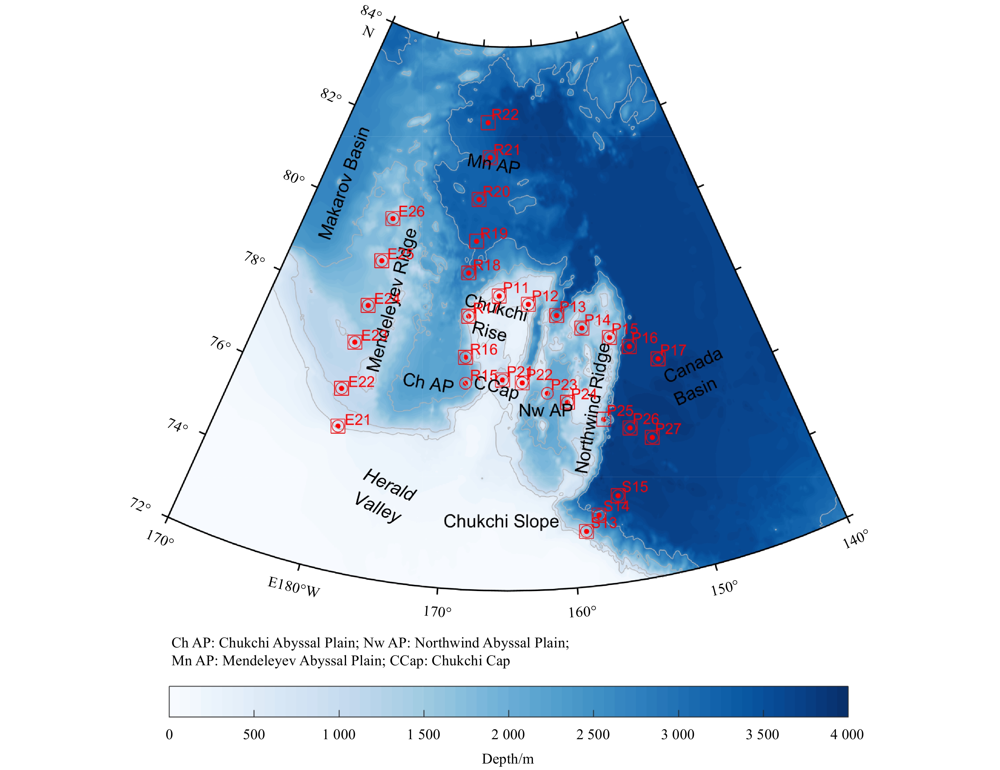
We defined five sections according to the CTD stations (Fig. 1). Section E lies on the Mendeleyev Ridge (MR). Section R is distributed from the Chukchi Cap (CCap) to the Mendeleyev Abyssal Plain (Mn AP) along the longitude of 170°W, with R15–R17 on the CCap and R18–R22 in the Mn AP. Sections P1 and P2 extend from the west of the CCap to the western Canada Basin (CB), with P11–P15 and P21–P25 on the CCap and P16–P17 and P26–P27 in the western CB. Section S is located from the Chukchi shelf (S13–S14) to the southern CB (S15).

Figure  1.  Hydrographic and turbulent stations of the 7th Chinese National Arctic Research Expedition in the Chukchi Borderland and Mendeleyev Ridge of the Arctic Ocean in the summer of 2016. CTD stations are marked as red dots, stations with quality sADCP data are marked as red squares, and VMP stations are marked as red circles. The colormap shows the bathymetry.

DownLoad: Full-Size Img PowerPoint

3. Results

3.1 Water mass

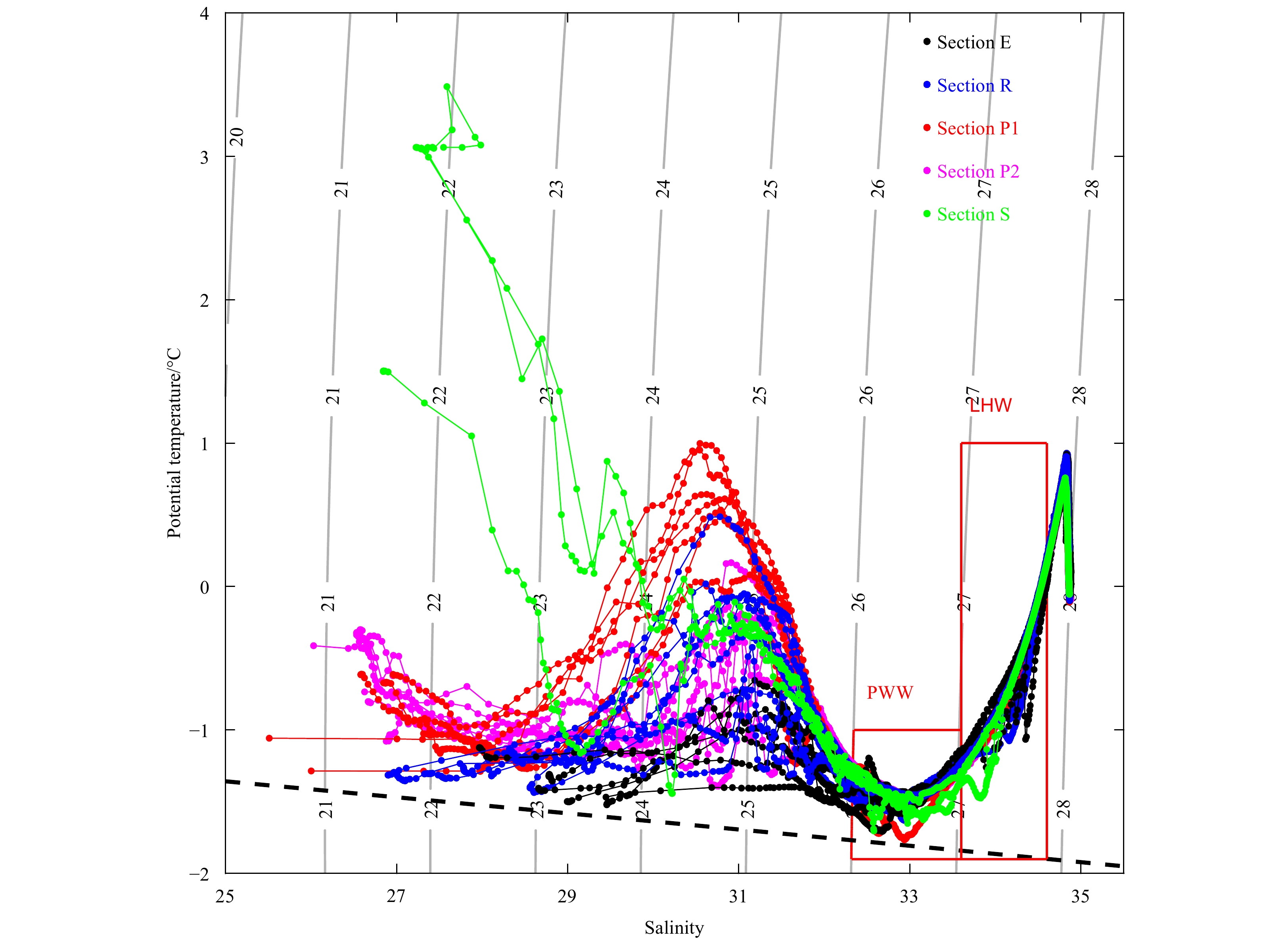
Figure 2 is the T-S diagram of all stations, and Fig. 3 shows the potential temperature, salinity, and buoyancy sections of Sections P1 and E, for identifying the water masses. The AW existed at the intermediate depths over the entire CBLMR, with a potential temperature maximum, which is defined as the Atlantic Water Core (AWC; Zhong and Zhao, 2014). In CBLMR, AW was carried by a circuitous boundary current, owning to its complex topography (Woodgate et al., 2007). The upper ocean overlying the AW shows a distinct spatial difference. Pacific Water extends horizontally over almost all the Chukchi Borderland, except on the MR. As Section P1 shows, there is a prominent temperature maximum in the subsurface layer, with a salinity range between 30 and 33, which is identified as Pacific Summer Water (PSW; Shimada et al., 2001; Timmermans et al., 2014). Same do Section R, Section P2 and Section S (not shown). There is also a temperature minimum between PSW and AW, with salinity centered at 33.1, which is Pacific Winter Water (PWW; Jones and Anderson, 1986; Itoh et al., 2012). Zhong et al. (2019) also identified PWW as the water mass between the isopycnal of 26.0 kg/m³ and 27.0 kg/m³. However, the potential temperature profile of Section E on the MR does not present a similar feature. The subsurface water on the MR was colder and saltier than the other sections. According to previous studies with CTD observations and additional nutrient and optical parameters, Jones et al. (1998) and Zhao et al. (2015) identified the subsurface water above AW on the MR as a mixing of Atlantic-origin and Pacific-origin water.

Figure  2.  T-S diagram of all stations.

DownLoad: Full-Size Img PowerPoint

Figure  3.  Potential temperature (a, b), salinity (c, d), and buoyancy frequency (e, f) sections of Sections P1 (left) and E (right). White dash lines are the isopycnals of 26 kg/m³ and 27 kg/m³.

DownLoad: Full-Size Img PowerPoint

In the Arctic Ocean, the pycnocline between the polar mixed layer and the Atlantic layer is commonly called the halocline (Coachman and Aagaard, 1974). With the existence of Pacific Water, the halocline in the Canadian Basin was divided into the upper halocline and lower halocline. The former was dominated by PSW and PWW, and the latter was defined as having a potential temperature of θ<0°C and salinity range of 33.6<S<34.6 (Rudels et al., 2004). Aksenov et al. (2011) also defined AW with 34.70≤S≤34.95, and halocline water with θ<0°C, S<34.70. The buoyancy frequency sections of both P1 and E show a peak between the subsurface layer and lower halocline water, and the depth of this peak corresponds well with the isopycnal of 27.0 kg/m³ and isohaline of 33.6. Therefore, we focus on the lower halocline water between the two isohalines of 33.6 and 34.6 to estimate the turbulent dissipation rate, diffusivity, and vertical heat flux from Atlantic Water to upper Pacific Water.

3.2 Richardson number

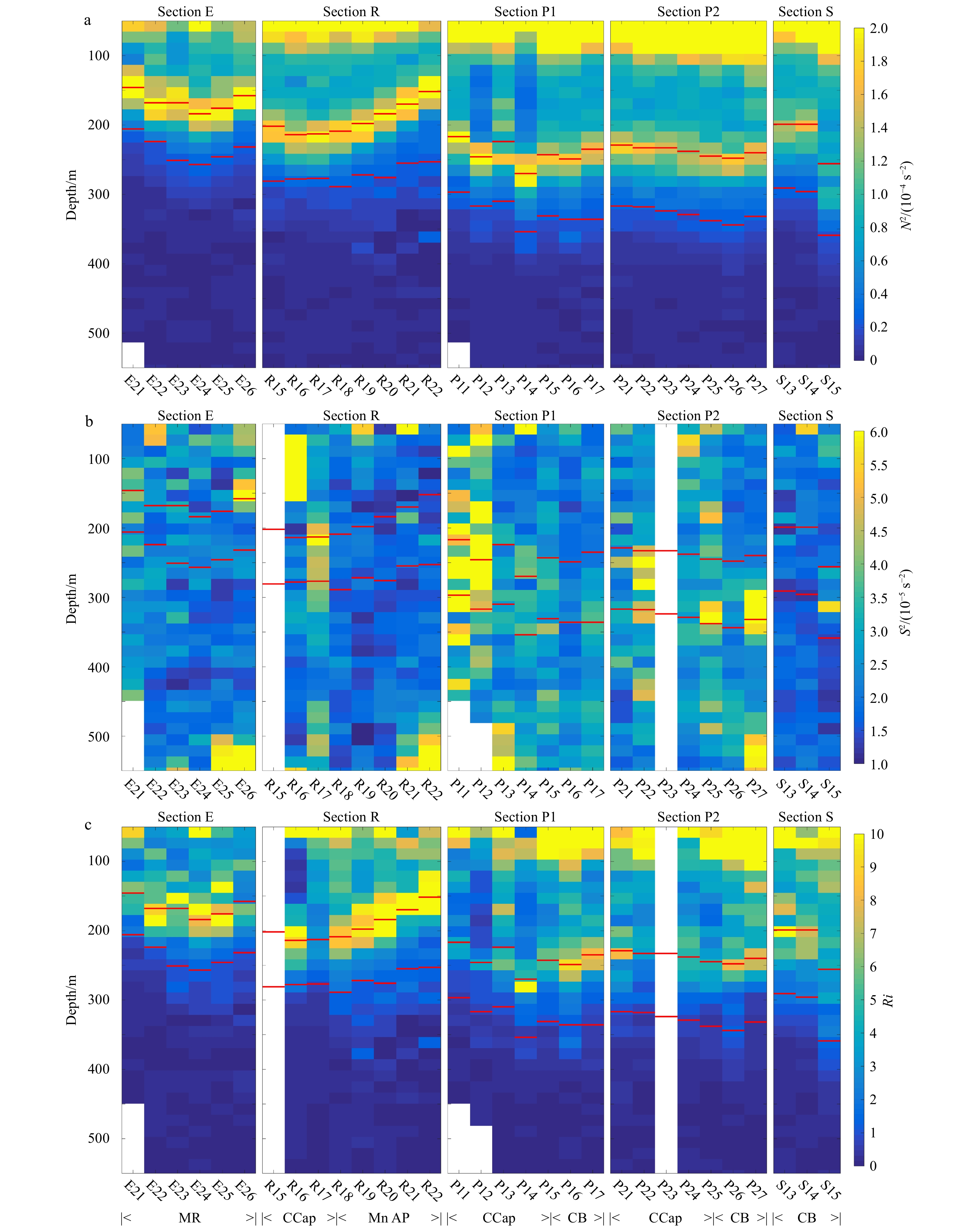
The buoyancy frequency (N²) characterizes the intensity of stratification, as $ {N}^{2}=-(g/\rho)(\partial \rho/\partial z) $, where g is the gravity acceleration, ρ is the density, and z is the vertical coordinate (upward is positive). Sectional snapshots of N² are shown in Fig. 4a. A distinct peak of N² exists just at the top of the lower halocline water. This strong stratification separated the lower halocline water from the upper ocean, and acted as a barrier to prevent upward and downward mixing. Regarding the depth of this stratification peak, it was shallowest in Section E on the MR, at approximately 170 m. From south to north of the MR, the depth of this stratification peak first deepens from E21 to E24, and then shallows from E24 to E26. The distribution of this stratification peak in Section R was similar to that in Section E, although the depth in Section R was slightly deeper (the mean depth was approximately 180 m). The stratification peak in Sections P1 and P2 was the deepest, with an average depth of 250 m. In addition, this stratification peak also showed spatial variation. The stratification peak on the MR (E21–E26), Mn AP (R18–R22), and northwest of CCap (P11–P14) was strongest, from 1.9×10^–4 s^–2 to 2.4×10^–4 s^–2. It was considerably smaller in the south and east of the CCap and western CB (P15–P17, P21–P27), from 1.3×10^–4 s^–2 to 1.7×10^–4 s^–2. Section S (S13–S15) showed the weakest stratification among all sections, from 1.0×10^–4 s^–2 to 1.6×10^–4 s^–2. The pattern revealed that the water closer to the central CB (Sections P1, P2, and S) was accompanied by weaker stratification.

Figure  4.  Buoyancy frequency N² (a), vertical shear S² (b) and Richardson number Ri (c) of each section. Upper red line is the isohaline of 33.6, and lower red line is the isohaline of 34.6.

DownLoad: Full-Size Img PowerPoint

Vertical shear S² was obtained from sADCP measurements as $ {S}^{2}={\left(\partial u/\partial z\right)}^{2}+{\left(\partial v/\partial z\right)}^{2} $, where u and v are the zonal and meridional currents respectively. As shown in Fig. 4b, S² was strongest at CCap, and the depth-averaged value in the LHW was 3.8×10^–5 s^–2 from western CCap to the western CB (Sections P1 and P2, R15–R17). In particular, at Stations R17, P11, P12, and P22 on the Chukchi Rise, S² was larger than 4.9×10^–5 s^–2. Accordingly, S² on the MR (E21–E26), Mn AP (R18–R22), and southern CB (S13–S15) was much weaker (1.6–3.3×10^–5 s^–2) than that at the CCap.

The Richardson number (Ri) was obtained from the buoyancy frequency over vertical shear, $ {R}{{i}}={N}^{2}/{S}^{2} $. As shown in Fig. 4c, most values of Ri in the LHW at the CCap were relatively smaller due to higher vertical shear, which implied that turbulent mixing from the AW to the upper ocean through the LHW at the CCap was more intensive than in other regions. The Ri in the LHW was relatively higher on the MR and Mn AP due to stronger stratification. The results supported that the shear instability was not significant with stronger stratification.

3.3 Dissipation rate, diapycnal diffusivity and vertical heat flux

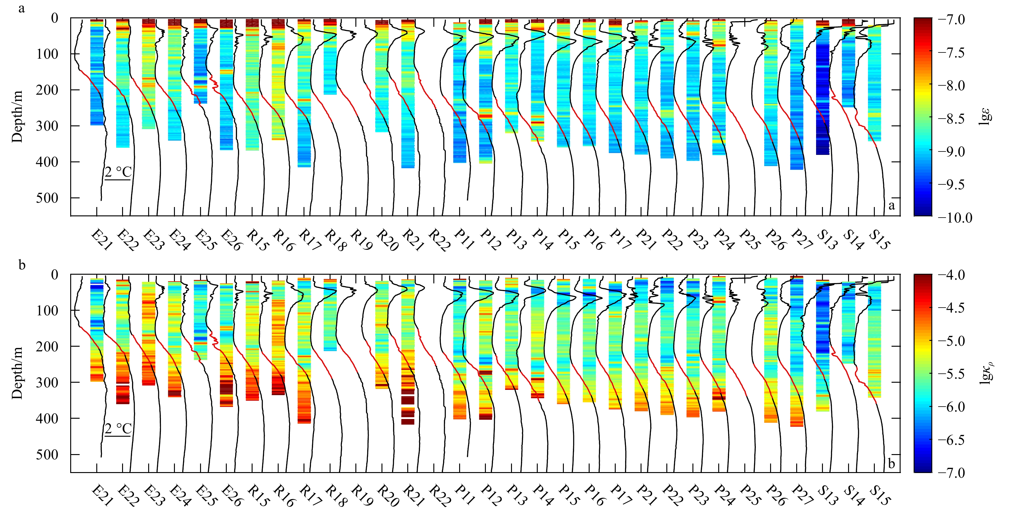
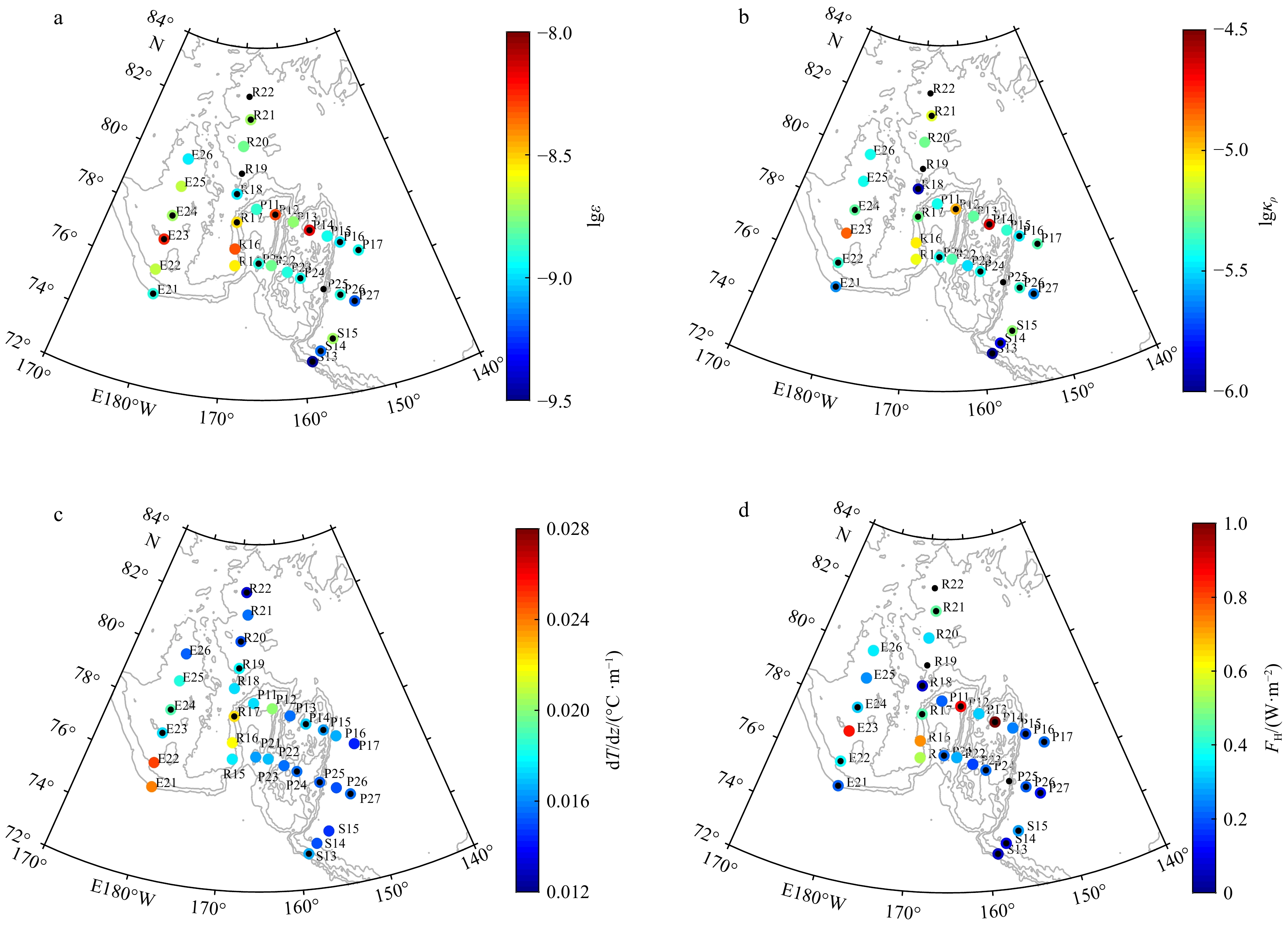
We used high-frequency VMP-200 shear data to obtain the dissipation rate of turbulent kinetic energy (ε), $ \varepsilon =\dfrac{15}{2}\nu \bar{{\left(\dfrac{\partial u}{\partial z}\right)}^{2}} $, where $ \nu $ is the kinematic viscosity (Fig. 5a). The shear variance was obtained by integrating the wavenumber spectrum of shear from 1 cycle per meter (cpm) to Kolmogoroff wave number based on the empirical mode from Nasmyth (1970). As Fig. 6a shows, the observed depth-averaged dissipation rate of the LHW in the western CB (P16–P17, P26–P27) ranged from 6.4×10^–10 W/kg to 1.2×10^–9 W/kg. However, in S15, the depth-averaged dissipation rate attained 2.0×10^–9 W/kg. It is slightly higher in Mn AP than CB with a mean value of 1.5×10^–9 W/kg. The results were close to but above the instrument noise level (10^–11 W/kg) and comparable with those of previous studies (Fer, 2009; Lenn et al., 2009; Guthrie et al., 2013; Rippeth et al., 2015; Zhong et al., 2018). The depth-averaged dissipation rates on the MR (E21–E26) and in the northwest CCap (R15–R17, P11–P14) were considerably higher than those in the deep basin, with a mean value of 2.4×10^–9 W/kg and 3.7×10^–9 W/kg, respectively.

Figure  5.  Profiles of dissipation rate (a) and diapycnal diffusivity (b) of each station. Vertical black curve line represents the potential temperature profile, and LHW in temperature profile is marked with red color. The unit of ε is W/kg, and the unit of κ_ρ is m²/s.

DownLoad: Full-Size Img PowerPoint

Figure  6.  Spatial distribution of depth-averaged dissipation rate ε (a), diapycnal diffusivity κ_ρ (b), temperature gradient dT/dt (c), and vertical heat flux F_H (d) in LHW for each section. The unit of ε is W/kg, and the unit of κ_ρ is m²/s.

DownLoad: Full-Size Img PowerPoint

Then, diapycnal diffusivity κ_ρ can be deduced from the dissipation rate ε as $ {\kappa }_\rho =0.2\varepsilon {N}^{-2} $ (Osborn, 1980; Gregg et al., 2018; Fig. 5b). The results of the depth-averaged diapycnal diffusivity κ_ρ in the LHW are shown in Fig. 6b. Depth-averaged κ_ρ in LHW is 4.3×10^–6 m²/s in the southwest CB (P17, P26–P27, S15), and 4.7×10^–6 m²/s in Mn AP, approximately 2 times larger than that estimated in the central CB (Lique et al., 2014) and numerical model (Zhang and Steele, 2007). It increases to 5.6×10^–6 m²/s on the MR (E21–E26), and 7.0×10^–6 m²/s on CCap (P11–P15, P21–P25, R15–R17), respectively. The mean value of depth-averaged κ_ρ of all section in the CBLMR in the LHW was 5.6×10^–6 m²/s. This value was comparable with the previous observation within the depth range of 200 m to 300 m in the same region in 2014 (Zhong et al., 2018), but about 4 to 5 times larger than that estimate in the central Canada Basin (Lique et al., 2014) and numerical model (Zhang and Steele, 2007).

Finally, we computed the vertical heat flux as $ {F}_{\mathrm{H}}=\rho {c}_{\mathrm{p}}\kappa \dfrac{\partial T}{\partial z} $, where ρ is the sea water density, c_p is the heat capacity of seawater, and κ is the vertical diffusivity. F_H is positive upward. Depth-averaged vertical heat fluxes are shown in Fig. 6d. In the southwest CB (S15, P17, P26–P27), the mean vertical heat flux in the LHW is 0.21 W/m². It is slightly higher in Mn Ap than in the CB, with a mean value of 0.30 W/m². These values of vertical heat flux in the deep basin corresponded well with previous studies (Timmermans et al., 2008; Lique et al., 2014; Zhong et al., 2018). The mean depth-averaged vertical heat flux of the LHW was 0.39 W/m² on the MR and 0.46 W/m² on the CCap, respectively. The observed maximum vertical heat flux of the LHW was 0.28 W/m² in S15 in the southern CB, 0.85 W/m² in E23 on the MR, and 1.3 W/m² in P14 on the CCap, which was ascribed to either strong surface (S15, E23, and P14) wind forcing or strong semidiurnal tidal energy (E23). However, the temperature gradient between the PSW and PWW is reversed, when compared with that it in the LHW. As a result, we suggest that the upward heat released from AW through the lower halocline could hardly contribute to the surface ocean.

3.4 Mechanisms of the diaypcnal mixing in LHW

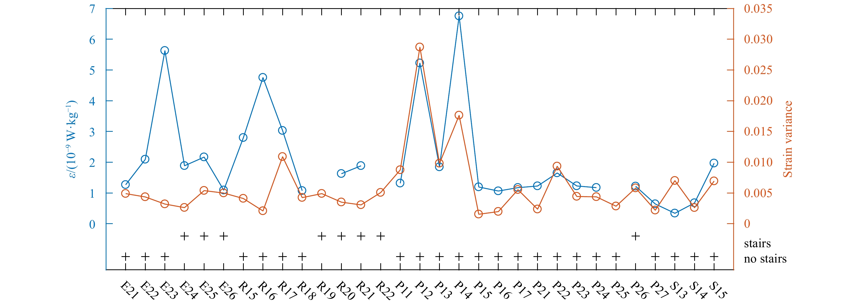
Carmack et al. (2015) summarized that two mechanisms —double diffusion and shear instabilities—were thought to be responsible for most upward diapycnal fluxes from AW. Double-diffusive staircases were observed in 8 stations, including P26 in the Canada Basin, E24–E26 on MR, and R19–R22 in Mn AP. Within them, 5 stations were measured by VMP. This staircase structure between PWW and AWC is believed to be maintained by double-diffusive convection, when colder and fresher Pacific water lies above warmer and salty Atlantic water (Timmermans et al., 2008). Here, we only focused on the double diffusion in LHW. The depth averaged dissipation rate in double-diffusive staircases in LHW ranges from 1.01×10^–9 W/kg to 1.57×10^–9 W/kg (Table 1). It is relatively smaller than that in most of other stations where there are no double-diffusive staircases.

Table  1.  Comparison of the depth averaged diffusivity between observation and parameterization where double diffusion occurred in LHW

Station name	Observed dissipation rate ε/(10–9 W·kg–1)	Diffusivity derived from observed dissipation rate κ/(10–6 m2·s–2)	Diffusivity based on double-diffusive theory κ/(10–6 m2·s–2)
E24	1.57	7.90	5.16
E26	1.14	6.69	6.49
R20	1.47	7.89	5.38
R21	1.44	9.55	5.90
P26	1.01	6.75	5.05

 | Show Table

DownLoad: CSV

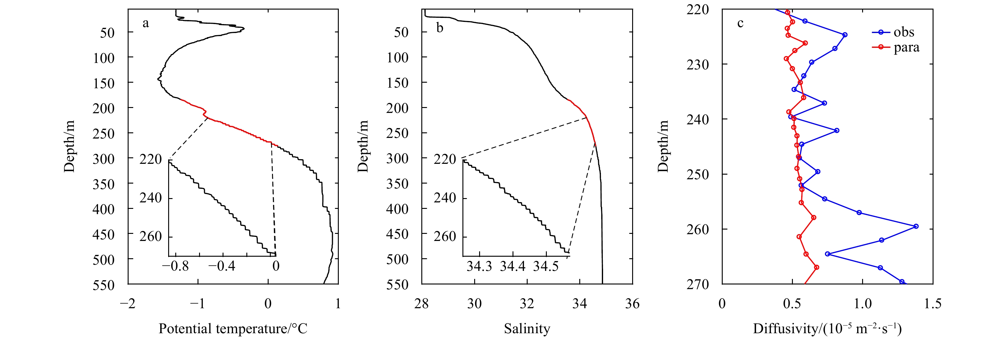
We also compared the diffusivity between VMP observation and parameterization. Diffusivity of double-diffusive can be described by a relationship of the form, k_T=k₀(1–R–R_ρ)^–3/2 with k₀=3.9×10^–6 m²/ s. R_ρ=βΔS/αΔθ is the density ratio, where α and β are thermal expansion coefficient and saline contraction coefficient, respectively, and ΔS and Δθ are changes in potential temperature and salinity across the stair interface (Shaw and Stanton, 2014b; Flanagan et al., 2014). As Fig. 7 and Table 1 show, the observed diffusivities in double-diffusive staircases ranged from 6.69×10^–6 m²/s² to 9.55×10^–6 m²/s². It was usually 1.3 to 1.6 times larger than it by the parameterization, except in E26. Generally, the double-diffusive staircase always represents weak diapycnal mixing.

Figure  7.  Profile of double diffusive staircase potential temperature (a), salinity (b), and diffusivity comparison between observation (blue) and parameterization (red) in R20 in Mn AP (c).

DownLoad: Full-Size Img PowerPoint

We further explored the underlying mechanism of the depth-averaged turbulent dissipation rate in the LHW with the internal wave activities, which can cause shear instability and lead to generation of turbulence. Halocline strain variance ($ \left\langle { {\xi }_{z}^{2} } \right\rangle $) is always considered as a surrogate for internal wave activity, which can be estimated from buoyancy $ {\xi }_{z}=\left({N}^{2}-{\bar{N}}^{2}\right)/{\bar{N}}^{2} $, where mean stratification $ {\bar{N}}^{2} $ is based on quadratic fits to each profile segment (Polzin et al., 1995; Kunze et al., 2006; Qiu et al., 2012). Herein, a segment of 20 m was applied. And we took the depth-averaged strain variance within the LHW. In general, the turbulent dissipation rate increases with the increasing strain variance (Fig. 8). For most stations, the strain variance in the LHW was less than 0.011. However, it reached 0.018 and 0.029 in P14 and P12, respectively. The turbulent dissipation rate and CTD-derived halocline strain variance were significantly correlated (at a confidence level of greater than 95%), with a correlation coefficient of 0.55 and p<0.003. This result demonstrates a close physical linkage between the turbulent mixing and internal wave activities.

Figure  8.  Depth-averaged dissipation rate (blue) and strain variance in lower halocline water (red) of each station. Black pluses mark where double-diffusive staircases were observed.

DownLoad: Full-Size Img PowerPoint

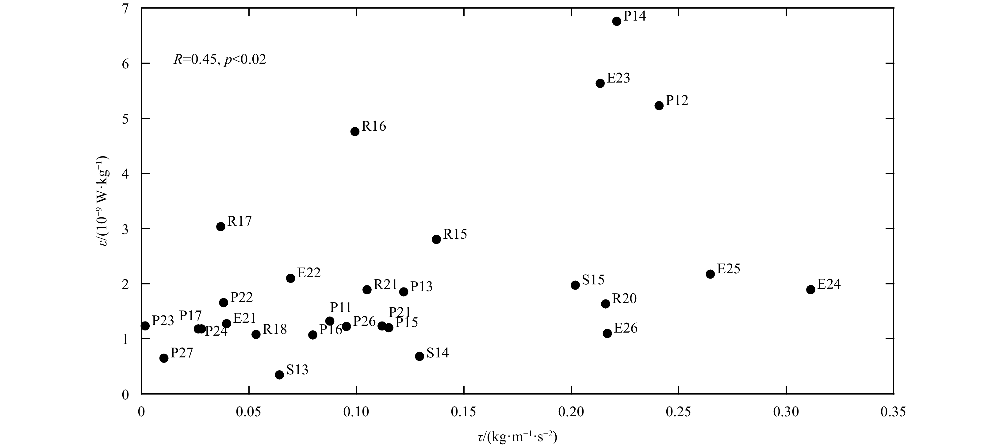
Wind and tides are two main sources of kinetic energy, involved in driving turbulent mixing in the ocean. Sea surface forcing by surface winds can contribute to deeper ocean turbulent mixing by generating near-internal currents within the surface mixed layer, which then penetrate downward (Nagasawa et al., 2000; Alford, 2003; Liu and Lozovatsky, 2012; Lincoln et al., 2016; Yang et al., 2017; Qiu et al., 2019). We further explored the connection between the turbulent dissipation rate and surface wind stress. The total surface stress of sea-ice-covered ocean in CBLMR at each station was calculated based on in situ 10 m surface wind, and sea ice concentration data derived from Advanced Microwave Scanning Radiometer 2 (AMSR2; Spreen et al., 2008), which was suggested by Yang (2009) as ${\mathord{\buildrel{\lower3pt\hbox{$\scriptscriptstyle\rightharpoonup$}} \over \tau } _{{\rm{total}}}}{\rm{ = }} $$ \left( {{{1 - }}\alpha } \right){\mathord{\buildrel{\lower3pt\hbox{$\scriptscriptstyle\rightharpoonup$}} \over \tau } _{{\rm{air-water}}}}{\rm{ + }}\alpha {\mathord{\buildrel{\lower3pt\hbox{$\scriptscriptstyle\rightharpoonup$}} \over \tau } _{{\rm{ice-water}}}}$, where $ \alpha $ is the average sea ice concentration around the station within a radius of less than 50 km. $ {\mathord{\buildrel{\lower3pt\hbox{$\scriptscriptstyle\rightharpoonup$}} \over \tau } _{{\rm{air-}} {\rm{water}}}} = {\rho _{{\rm{air}}}}{C_{\rm{d}}}\left| {{{\mathord{\buildrel{\lower3pt\hbox{$\scriptscriptstyle\rightharpoonup$}} \over u} }_{\rm{s}}}} \right|{\mathord{\buildrel{\lower3pt\hbox{$\scriptscriptstyle\rightharpoonup$}} \over u} _{\rm{s}}} $, where $ {\rho }_{\mathrm{a}\mathrm{i}\mathrm{r}}=1.25\;\mathrm{k}\mathrm{g} / {\mathrm{m}}^{3} $ is the air density, $ C_{\text{d}}\text{=0.001\;25} $ is the drag coefficient, and $ {\mathop u \limits^{\rightharpoonup}}_{\text{s}} $ is 10 m surface wind. $ {\mathord{\buildrel{\lower3pt\hbox{$\scriptscriptstyle\rightharpoonup$}} \over \tau } _{{\rm{ice - water}}}} = {\rho _{{\rm{water}}}}{C_{{\rm{iw}}}}\left| {({{\mathord{\buildrel{\lower3pt\hbox{$\scriptscriptstyle\rightharpoonup$}} \over u} }_{{\rm{ice}}}} - {{\mathord{\buildrel{\lower3pt\hbox{$\scriptscriptstyle\rightharpoonup$}} \over u} }_{{\rm{ocean}}}})} \right|({\mathord{\buildrel{\lower3pt\hbox{$\scriptscriptstyle\rightharpoonup$}} \over u} _{{\rm{ice}}}} - {\mathord{\buildrel{\lower3pt\hbox{$\scriptscriptstyle\rightharpoonup$}} \over u} _{{\rm{ocean}}}}) $, where $ \rho _{\text{water}}\text{=1\;024}\;\text{kg} / {\text{m}}^{{3}} $ is the sea water density, $ C_{\text{iw}}\text{=0.005\;5} $ is the ice-water drag coefficient (Hibler III, 1979), and $ {\mathop u \limits^{\rightharpoonup}}_{\text{ice}}-{\mathop u \limits^{\rightharpoonup}}_{\text{ocean}} $ is simplified as 2% of surface wind (Thorndike and Colony, 1982). The connection between the turbulent dissipation rate and surface wind stress was evident, with a correlation coefficient of 0.45 and p<0.02 (Fig. 9). In P12, P14, and E23, the observed surface wind velocity was more than 10 m/s and with surface stress ${\mathord{\buildrel{\lower3pt\hbox{$\scriptscriptstyle\rightharpoonup$}} \over \tau } }_{\mathrm{t}\mathrm{o}\mathrm{t}\mathrm{a}\mathrm{l}} > 0.2$, which resulted in a dissipation rate more than 5×10^–9 W/kg. For most stations where $ {\mathord{\buildrel{\lower3pt\hbox{$\scriptscriptstyle\rightharpoonup$}} \over \tau } }_{\mathrm{t}\mathrm{o}\mathrm{t}\mathrm{a}\mathrm{l}}<0.15 $, the turbulent dissipation rate was no more than 2×10^–9 W/kg. However, for some stations, such as E25 and E24 on the MR with $ {\mathord{\buildrel{\lower3pt\hbox{$\scriptscriptstyle\rightharpoonup$}} \over \tau } }_{\mathrm{t}\mathrm{o}\mathrm{t}\mathrm{a}\mathrm{l}}>0.25 $, the dissipation rate remained at a lower level of ~2×10^–9 W/kg, despite stronger surface wind forcing. To some extent, this still implies that the surface wind supplies energy to turbulent mixing at intermediate depths.

Figure  9.  Depth-averaged dissipation rate in lower halocline water and surface wind stress.

DownLoad: Full-Size Img PowerPoint

Tides also play a key role in global ocean circulation through the supply of mechanical energy to turbulence that stirs the ocean, thereby promoting mixing (Munk and Wunsch, 1998; Simmons et al., 2004; Lozovatsky et al., 2013; Yang et al., 2017). Rippeth et al. (2015) showed that the enhanced levels of turbulent dissipation rate observed over the Arctic Ocean continental shelf break are correlated to the rate of conversion of tidal energy. CBLMR lies slightly north of the critical latitude, at which the local inertial period matches the period of the semidiurnal tides (M₂ and S₂). To clarify the connection between the turbulent dissipation rate and the intensity of the regional semidiurnal tides, we extracted the M₂ and S₂ tidal current information from the output of the Arctic Ocean Tidal Inverse Model (Arc5km2018, Erofeeva and Egbert, 2020). We calculated the depth-average tidal energy as $ {{E}}_{\text{TK}} = \dfrac{1}2 \rho \left({{u}}^2+{{v}}^2\right) $, where $ \rho $ is the seawater density, and u and v are the model outputs of the tidal velocities. The results show that the turbulent dissipation rate and semidiurnal tidal energy are also well correlated, with a correlation coefficient of 0.44 and p<0.02 (Fig. 10). The semidiurnal tide is relatively strong at stations on the MR and in the western of CCap, leading to a larger turbulent dissipation rate. In western CB and Mn AP, where semidiurnal tide is weak, the dissipation rate is relatively smaller. Thus, the semidiurnal tide also significantly contributes to turbulent mixing in the LHW.

Figure  10.  Depth-averaged dissipation rate in lower halocline water and semidiurnal tidal energy. The unit of ε is W/kg, and the unit of E_TK is J/m.

DownLoad: Full-Size Img PowerPoint

4. Summary

Oceanic vertical mixing of the LHW above the AW was investigated using hydrographic and turbulent data over the CBLMR during the summer of 2016. The shipboard ADCP showed that the vertical shear in LHW was remarkable over the CCap, moderate over the MR, and relatively weak in the surrounding deep basin.

The observed depth-averaged dissipation rate of the LHW ranged from 6.4×10^–10 W/kg to 1.2×10^–9 W/kg in the west Canada Basin, approximately 1.5×10^–9 W/kg in the Mn AP, 2.4×10^–9 W/kg on the MR, and 3.7×10^–9 W/kg in the northwest of Chukchi Cap. Correspondingly, the depth-averaged vertical heat flux is 0.21 W/m² in the southwest Canada Basin, 0.30 W/m² in Mn Ap, 0.39 W/m² on MR, and 0.46 W/m² on the Chukchi Cap. However, in the presence of PWW, the upward heat released from Atlantic Water through the lower halocline could hardly contribute to the surface ocean.

Two mechanisms—double diffusion and shear instability—of the turbulent mixing in LHW were investigated. The double diffusion were observed in 8 stations, and always accompanied by weak mixing with dissipation rate range from 1.01×10^–9 W/kg to 1.57×10^–9 W/kg. And, there is a significant connection between the dissipation rate and strain variance of the LHW, which indicates that the mixing in LHW induced by shear instabilities could be ascribed to internal wave activities. In addition, both surface wind stress and semidiurnal tidal energy have considerable contribution to the turbulent mixing in the LHW.

Acknowledgements

We thank the research groups of the 7th Chinese National Arctic Research Expedition for assistant of collecting the CTD, sADCP, VMP, and meteorological data. The sea ice concentration data is downloaded from https://seaice.uni-bremen.de/sea-ice-concentration/amsre-amsr2/#Data_Archive. The Arctic Ocean Tidal Inverse Model is from http://people.oregonstate.edu/~erofeevs/Arc.html.