Hainan Institute of Zhejiang University, Sanya 572024, China
2.
Ocean College, Zhejiang University, Zhoushan 316021, China
Funds:
The 2022 Research Program of Sanya Yazhou Bay Science and Technology City under contract No. SKJC-2022-01-001; the Project of Sanya Yazhou Bay Science and Technology City under contract No. SCKJ-JYRC-2022-47; the National Natural Science Foundation of China under contract No. 41806019; the Natural Science Foundation of Hainan Province under contract No. 121MS062; the National Natural Science Foundation of China under contract Nos 42006008 and 41876031; the National Key Research and Development Plan of China under contract No. 2016YFC1401603; the Research Startup Funding from Hainan Institute of Zhejiang University under contract No. HZY20210801.
Using observational data from multiple satellites, we studied seasonal variations of the shape and location of the Luzon cold eddy (LCE) northwest of Luzon Island. The shape and location of the LCE have obvious seasonal variations. The LCE occurs, develops, and disappears from December to April of the next year. During this period, the shape of the LCE changed from a flat ellipse to a circular ellipse, and the change in shape can be reflected by the increase of the ellipticity of the LCE from 0.16 to 0.82. The latitude of center location of the LCE changes from 17.4°N to 19°N, and the change in latitude can reach 1.6°. Further study showed that seasonal variation of the northeast monsoon intensity leads to the change in the shape and location of the LCE. The seasonal variation of the LCE shape can significantly alter the spatial distribution of the thermal front and chlorophyll a northwest of the Luzon Island by geostrophic advection.
The South China Sea (SCS) is the largest semi-closed marginal sea in the Northwest Pacific (NWP). To the north, west, and south it is surrounded by continents and islands, while to the east it is separated from the NWP by Taiwan Island and the Philippines Islands (Fig. 1). The SCS is situated in the East Asian monsoon regime, and its large-scale ocean circulation is mainly controlled by monsoon (Chu et al., 1999; Hwang and Chen, 2000; Qu, 2000; Liu et al., 2004). In summer, prevailing southwest monsoon cause cyclonic (anticyclonic) circulation in the north (south) of the SCS; in winter, prevailing northeast monsoon cause cyclonic circulation in the whole SCS basin. In addition to the East Asian monsoon, the ocean circulation in the SCS is also affected by the intrusion of the Kuroshio through the Luzon Strait (LS) (Jia and Liu, 2004; Zhang et al., 2017). The Kuroshio can invade the SCS in the form of “Leak”, “Loop”, and so on, and can significantly affect the temperature-salt structure and ocean circulation in the north of the SCS (Caruso et al., 2006; Nan et al., 2011, 2015; Zhang et al., 2017).
Figure
1.
Topographic distribution of the South China Sea and winter climatological mean distribution of sea level anomaly (SLA) and wind vectors. The filling contour represents SLA (unit: 10−2 m). The arrows represent wind vectors (unit: m/s). The black solid line represents the −0.08 m contour of SLA. The red box encompasses 14.625°–19.875°N, 116.125°–121.125°E, which represents the region northwest of Luzon Island. HI: Hainan Island, LI: Luzon Island, TI: Taiwan Island.
The LS, located between the Luzon Island and Taiwan Island, is an important gap for energy and particle between the SCS and NWP (Nan et al., 2015; Sun et al., 2022). Affected by topography, monsoon and the Kuroshio, the dynamics process in the LS is extremely complex. Due to the special geographical topography of the LS, the monsoon and Kuroshio will interact with the topography, resulting in obvious local ocean phenomena (Qu, 2000; Wang et al., 2008; Sun et al., 2016a, b). The Luzon cold eddy (LCE) is one of the important local ocean phenomena northwest of the Luzon Island, and was first recorded in Nitani (1970). It occurs northwest of Luzon Island in boreal winter (Fig. 1), first appears in late autumn, peaks from December–January, and decays in early spring (Qu, 2000). Its intensity increases and then decreases from late autumn to early spring, and the maximum occurs between December and January (Qu, 2000; Wang et al., 2012). The LCE strengthens (weakens) during La Niña (El Niño) years (Zheng et al., 2007; Sun et al., 2015; He et al., 2016; Deng et al., 2022). Blocked by Luzon Island, the northeast monsoon produces positive wind stress curl in the northwest of Luzon Island, which then leads to the generation of the LCE (Wang et al., 2008; Sun et al., 2015).
LCE contributes to the complex dynamic environment and plays an important role in marine ecosystem in the SCS. LCE contributes to upwelling and then is beneficial to winter blooms of primary production (Shaw et al., 1996; Tang et al., 1999; Wang et al., 2010; Lu et al., 2015). Due to ocean advection of the LCE, the cold (warm) water is located in its northwest (southeast) part, forming a thermal front northwest of Luzon Island (Belkin and Cornillon, 2003; Wang et al., 2012; Sun et al., 2015). At the same time, the LCE is a quasi-stable and excellent object to study the characteristics of mesoscale eddy (Wang et al., 2012). Therefore, full understandings of the LCE are valuable for understanding the dynamics process and mesoscale eddies of the SCS.
Although a substantial amount of research on the LCE exist, we re-examined the LCE because of its importance, and found that seasonal variation of the shape and location of the LCE were significant and had an important impact on the marine environment such as spatial distribution of thermal front and chlorophyll a (Fig. 2). Previous studies mainly studied the statistical characteristics, formation mechanism and impact on the marine environment of the LCE in the climatological state (Wang et al., 2003, 2008, 2012; Sun et al., 2015). The study of seasonal variation is less probed. Although Sun and Liu (2011) pointed out that the LCE had a double eddy structure and studied the intraseasonal variation of geostrophic vorticity of the LCE structure northwest of the Luzon Island, seasonal variations of the other parameters such as shape and location of the LCE were not involved. To the best of our knowledge, it is unclear that seasonal variations of shape and location of the LCE. In order to systematically solve the question above, we will study the seasonal variations characteristic of shape and location of the LCE, its dynamic mechanism, and its impact on the marine environment in this paper. The rest of this paper is organized as follows: Section 2 briefly introduces the data and methods, Section 3 presents the research results, Section 4 provides a discussion, and Section 5 provides a conclusion.
Figure
2.
Seasonal variations in the shape and location of the Luzon cold eddy (LCE). The filling contour represents sea level anomaly (SLA). The thick black solid line represents the edge of the LCE. The thick red solid line represents the edge of the fitting ellipse for the LCE. The black star represents the center location of the LCE. The red star, located at 21.875°N, 118.375°E southwest of Taiwan Island, represents the location along which the SLA gradient north of the South China Sea is defined. The white solid line represents the distance between the black star and red star.
Satellite-observed sea level anomaly (SLA) and geostrophic current were obtained from the Copernicus Marine Environment Monitoring Service (CMEMS). The dataset merged data from all altimeter missions including Sentinel-3A/B, HY-2A, Jason-3, Cryosat-2, Jason-1, TOpeX/Poseidon, OSTM/Jason-2, Envisat, GFO, and ERS-1/2. The datasets contain one near-real product and one delayed-time product which is used in this paper. The delayed-time datasets have been intercalibrated, providing high-precision and long-time series data from January 1, 1993, to August 2, 2021 (Pujol, 2022). The spatial and temporal resolution of the delayed-time datasets are 0.25°×0.25° and 1 day, respectively. The datasets contain aliases from coastal waves and tides signals on the shallow shelf, so we masked out the data for ocean regions with a water depth of fewer than 200 m.
Chlorophyll a concentration datasets were provided by the Moderate Resolution Imaging Spectroradiometer (MODIS) of the National Aeronautics and Space Administration (NASA). They have a temporal resolution of 1 day and a spatial resolution of 0.25°×0.25°. The datasets are calculated using an empirical relationship derived from in situ measurements of chlorophyll a and remoting sensing reflectances in the blue-to-green region of the visible spectrum (Hu et al., 2012).
Cross-Calibrated Multi-Platform (CCMP) version 2.0 ocean vector wind datasets were from Remote Sensing Systems. The CCMP dataset merged satellite remote sensing observation data, in situ observation data, and model wind data using multiple analysis methods. It provides global coverage data from August 1987 to present, with a spatial resolution of 0.25°×0.25° and a temporal sampling frequency of 6 h (Atlas et al., 2011; Mears et al., 2019).
Optimum Interpolation Sea Surface Temperature (OISST) data were provided by National Centers for Environmental Information (NCEI). The dataset incorporates observations from different platforms: ships, buoys, satellites and Argo floats into a regular global grid. Interpolation was used to fill gaps on the grid. Ship and satellite observation data were referenced to buoy observation data to compensate for platform differences and sensor biases. The OISST dataset provides a global coverage from January 1, 1982 to present, with a spatial resolution of 0.25°×0.25° and a temporal sampling frequency of 1 day (Huang et al., 2021).
2.2
Methods
2.2.1
SOM method
The LCE northwest of Luzon Island has complex spatiotemporal characteristics. In this study, in order to extract the representative spatial mode of the LCE, we introduced the self-organizing map (SOM) method. Based on unsupervised learning, SOM is an artificial neural network, and is an effective method for classification and feature extraction (Kohonen, 2001; Tsui and Wu, 2012). This method gathers similar features into a class and can also be regarded as a clustering method. It has been applied to many oceanographic studies and achieved good results (Liu et al., 2006; Liu and Weisberg, 2007; Tsui and Wu, 2012; Sun et al., 2016a, 2018; Gu et al., 2018; Lu et al., 2022).
The parameters such as lattice, training method, map shape, initialized weight and map size need to be specified before the training process of SOM. In this study, the tunable parameters were chosen based on the reference of Liu et al. (2006), which gave a practical process for choosing tunable parameters. The parameter of map size is obtained through tests according to actual situation of the LCE. In Fig. 2, the variation of the LCE is mainly manifested in the variation of shape and location, and the variation of shape and location are phase locked. The closer the shape of the LCE is to the circle, the farther north the location of the LCE is. Therefore, a map size of 1 × 2 was chosen in this study. A series of tests with different sizes such as 1 × 3, 2 × 2, and 2 × 3 were run, respectively. Although the patterns in the larger map size of the SOM provided more details about the LCE, the patterns of the LCE were very similar to the ones with the map size of 1 × 2.
Using minimum Euclidean distance for input data, SOM gives a best-matching unit (BMU), which records the category of each pattern of the LCE. A time series of BMU can reflect the evolution process of every pattern of the LCE and can be used to calculate the occurrence frequency of every pattern of the LCE.
2.2.2
Definition of ellipticity and included angle of α fitting ellipse for the LCE
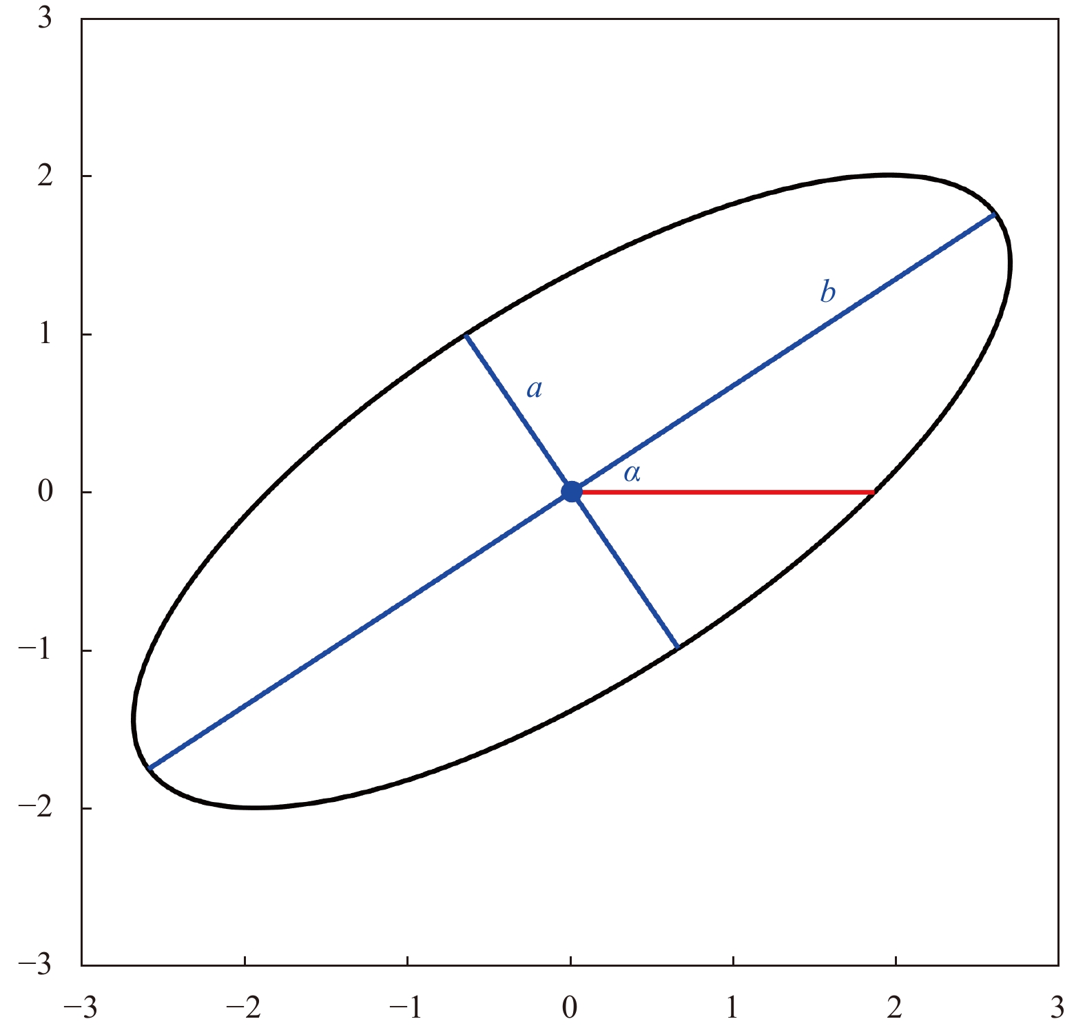
Figure 3 is a schematic of a fitting ellipse for the LCE. The ellipticity of the LCE ellipse is defined as the ratio of the minor axis to the major axis of ellipse. The formula can be expressed as $\mathrm{e}\mathrm{l}\mathrm{l}\mathrm{i}\mathrm{p}\mathrm{t}\mathrm{i}\mathrm{c}\mathrm{i}\mathrm{t}\mathrm{y}={a}/{b}$. The included angle $ \alpha $ is defined as the angle between the major axis of the ellipse and the due east direction. The definition of ellipticity and included angle of the LCE was used to characterize the shape and rotation direction of the LCE.
Figure
3.
Schematic diagram of the fitting ellipse for the Luzon cold eddy. a and b represent the minor axis and major axis of the ellipse, respectively. $ \alpha $ represents the included angle.
The LCE is essentially a mesoscale eddy. Its particularity lies in its proximity to land and its quasi-stable state. We identify the LCE according to the following four criteria (Wang et al., 2003; Sun et al., 2016a): (1) the presence of closed SLA contours; (2) the center position of the LCE is over water deeper than 200 m; (3) the SLA difference between its center and its outermost contour is greater than 4×10⁻² m (Roemmich and Gilson, 2001); and (4) the contour closest to land represents the edge of the LCE. The 3rd criterion was chosen because the satellite measurement error of the SLA is around 2×10⁻²–3×10⁻² m (Ducet et al., 2000). The identification method of the LCE was applied in identifying the outermost edge and shape of the LCE.
where GM is the gradient magnitude of SST; T is the SST; and x, y are the conventional east-west and north-south Cartesian coordinates, respectively. We chose 0.1℃/(10 km) as the threshold of the thermal front because the 0.1℃/(10 km) contour is a good reflection of the shape variation of the thermal front northwest of Luzon Island. We ran a series of tests with different thresholds such as 0.09℃/(10 km), 0.11℃/(10 km), and 0.12℃/(10 km). Our conclusions in this study are consistent. The definition of the thermal front was used to characterize the spatial range and intensity of thermal front northwest of the Luzon Island.
3.
Results
3.1
Seasonal variation of the LCE
3.1.1
Seasonal variation of the shape of the LCE
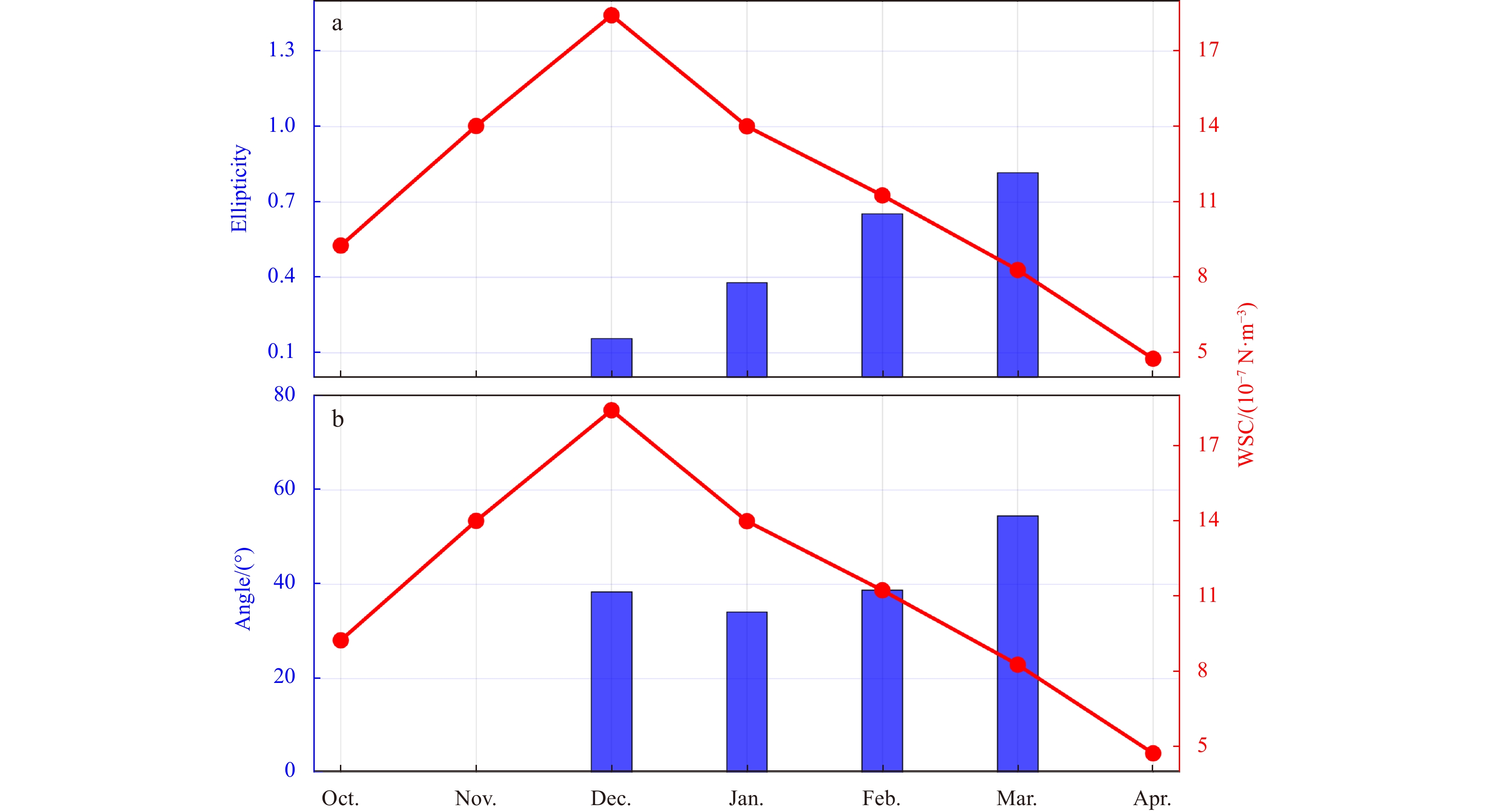
Based on satellite-observed SLA data and the LCE identification method described in the Section 2.2.3 to identify the LCE, we found that the shape of the LCE changed from a flat ellipse to a circular ellipse from December to March (Fig. 2). Figure 4 gives the seasonal variation of the shape of the LCE. Figure 4a shows that the ellipticity of the LCE increases gradually from 0.16 to 0.82 as the shape of the LCE changes from a flat ellipse to a circular ellipse. Figure 4b shows that the included angle decreases from 38.4° to 34.1° during December–January, and then increases from 34.1° to 54.5° during January–March, which indicates that the LCE rotates clockwise in the development stage (December–January), and then rotates counterclockwise in the recession stage (January–March).
Figure
4.
Correspondence between ellipticity of the fitting-ellipse of the Luzon cold eddy (LCE) and intensity of wind stress curl (WSC) northwest of Luzon Island (a); correspondence between the included angle of the fitting-ellipse of the LCE and WSC northwest of Luzon Island (b).
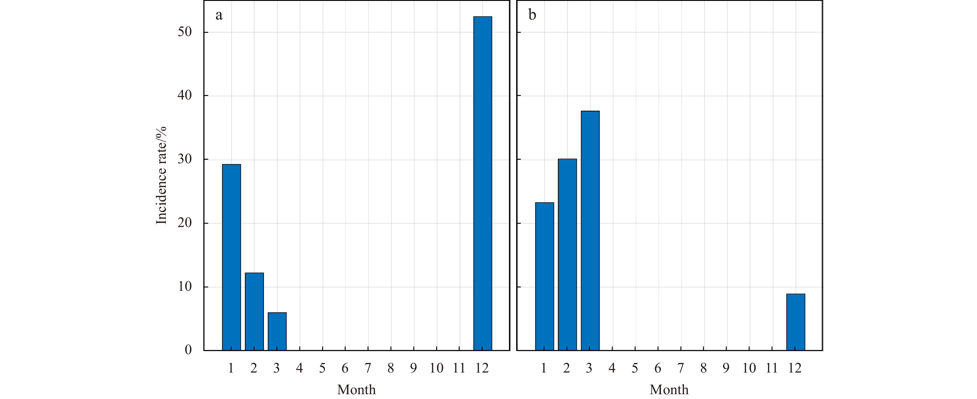
To extract more representative features of the seasonal variation of the LCE, we applied the SOM method to extract the temporal and spatial variation of the LCE. Figure 5 shows that the LCE has two main spatial structures. One is approximately elliptical (Fig. 5a) and the other is approximately circular (Fig. 5b). These are defined as the elliptical mode and the circular mode, respectively. Figure 6 shows that the elliptical (circular) mode of the LCE occurred mainly in December and January (February and March). This further verifies the seasonal variations in the shape of the LCE. The shape of the LCE was a flat (circular) ellipse in early winter (late winter and early spring).
Figure
5.
Two spatial patterns from self-organizing map analysis. a. Elliptical mode of the Luzon cold eddy (LCE); b. circular mode of the LCE. White numbers in each panel denote the incidence rate of the corresponding pattern. The black thick solid line represents the edge of the LCE. The interval between isolines is $ 5 \times {10}^{-3} $ m. SLA: sea level anomaly.
Figure
6.
Distribution of incidence rate of different spatial modes of the Luzon cold eddy. a. Distribution is for elliptical mode; b. Distribution is for circular mode.
3.1.2
Seasonal variation of the location of the LCE
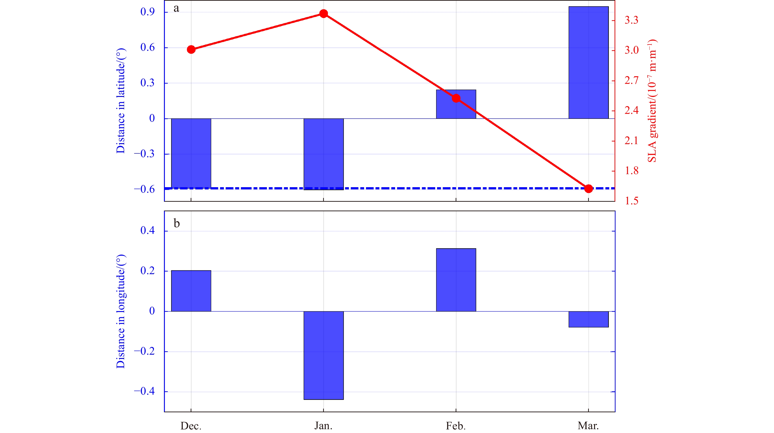
Based on satellite-observed SLA data and the LCE identification method described in the Section 2.2.3 to identify the LCE, we found that the center location of the LCE moves gradually north from December to March (Fig. 2). Figure 7 quantifies the seasonal variation of the location of the LCE. Figure 7a shows that the distance in latitude changes from −0.59° to −0.6° during December–January and changes from −0.6° to 1° during January–March, a difference of 1.6° latitude. The mean value of the latitude of the center location is 18°N, and the latitude of the LCE changes from 17.4°N to 19°N. Seasonal variation of the distance in longitude of the LCE shows no obvious pattern (Fig. 7b).
Figure
7.
Correspondence between distance of the center location of the Luzon cold eddy (LCE) and sea level anomaly (SLA) gradient north of the South China Sea. The SLA gradient is obtained by dividing the difference between the SLA at the red star and the black star by the corresponding distance in Fig. 2. a. In latitude, the mean latitude of the center location of the LCE is 18°N. b. In longitude, the mean longitude of the center location is 118.6°E.
The center of the elliptical (circular) mode of the LCE extracted by the SOM method was relatively south (north), and was located in 16.9°N, 118.1°E (18.4°N, 118.4°E) (Fig. 5), and the elliptical (circular) mode mainly occurred in December and January (February and March). This further verifies the seasonal variations in the location of the LCE. The center location of the LCE was relatively south (north) in early winter (late winter and early spring).
3.2
Dynamic mechanism of seasonal variation of the LCE
3.2.1
Dynamic mechanism of seasonal variation of the LCE shape
The formation of the LCE is related to the topographic wind stress curl northwest of Luzon Island, which also is one of main ocean dynamic processes northwest of Luzon Island (Qu, 2000; Wang et al., 2008). Therefore, we discussed the role of topographic wind stress curl northwest of Luzon Island in the seasonal variations of the LCE shape. Figure 4a shows that the shape of the LCE changes from a flat ellipse to a circular ellipse from December to March, and shows that the intensity of the wind stress curl northwest of Luzon Island weakens from December to March. There is a good correspondence between the shape of the LCE and the intensity of the wind stress curl. We inferred that the variation of the LCE shape was caused by the variation of the wind stress curl intensity. The smaller the intensity of wind stress curl northwest of Luzon Island, the closer the shape of the LCE is to the circle.
In order to verify the hypothesis above, we introduced the following extremum method. Figure 8 shows that the location of the positive wind stress curl northwest of Luzon Island is almost unchanged from October to April. Therefore, we can use the time series of the wind stress curl surrounded by the solid black line in Fig. 8 as the intensity index of wind stress curl (Fig. 9a). We composited SLA based on the days when the positive and negative intensity index values are more than one standard deviation away from the mean. Figure 9b (Fig. 9c) shows that the LCE is approximately elliptic (circular) when the wind stress curl northwest of Luzon Island is strong (weak). The process can be described as follow. Under the force of wind stress curl, the initial shape of the LCE must be consistent with the spatial shape of the wind stress curl northwest of Luzon Island. The shape of the wind stress curl is a northeast to southwest ellipse, so the shape of the LCE is flat elliptical in December. With the weakening of the wind stress curl, the LCE is no longer bound by the wind stress curl and gradually return to a circular ellipse in March.
Figure
8.
Seasonal variation in the wind stress curl (WSC) northwest of Luzon Island. The black solid line represents the climatological mean location of the WSC.
Figure
9.
Correspondence between Luzon cold eddy (LCE) and wind stress curl (WSC) northwest of Luzon Island from winter 1993 to winter 2020. Winter is defined as the period from December to March. a. Daily variation in the WSC. The upper (lower) red dotted line represents the sum (difference) of the one-time standard deviation and the average value of the time series, and the days when the time series is bigger (smaller) than the upper (lower) red dotted are defined as positive (negative) index days. b. Composition of sea level anomaly (SLA) for positive index days, and the thick black solid line represents the −0.08 m contour of SLA. The thick black (red) solid line represents the edge of the LCE (the fitting ellipse for the LCE), whose ellipticity is 0.26 (0.69). The black star represents the center location of the LCE. The red star, located at 21.875°N, 118.375°E, southwest of Taiwan Island, represents the location along which the SLA gradient north of the South China Sea is defined. The white solid line represents the distance between the black star and red star. c. Same as b, except for negative index days, and the thick black solid line represents the −0.06 m contour of SLA. The thick black (red) solid line represents the edge of the LCE (the fitting ellipse for the LCE), whose ellipticity is 0.69.
3.2.2
Dynamic mechanism of seasonal variation of the LCE location
The movement of water body in the ocean is mainly related to the pressure gradient. Therefore, we discussed the pressure gradient in the seasonal variation of the LCE location. Figure 7a shows that the LCE moves south from December to January, and then moves north from January to March, and shows that gradient of SLA north of the SCS increases from December to January, and then decreases from January to March. There is a good correspondence between distance variation of the LCE in latitude and the gradient of SLA north of the SCS. We inferred that location variation of the LCE was caused by the variation of the gradient of SLA north of the SCS. The smaller the gradient of SLA north of the SCS, the more southward the location of the LCE.
Although the Kuroshio can invade the north of the SCS through the LS in winter, dynamic height of the SCS, especially at the LCE, is still mainly controlled by the northeast monsoon (Qu, 2000; Liu et al., 2004). Therefore, the SLA gradient north of the SCS as is shown in Fig. 2 is mainly controlled by northeast monsoon (Qu, 2000). The SLA gradient north of the SCS in Fig. 9a (Fig. 9b) is 3.01×10⁻⁷ m/m (2.02×10⁻⁷ m/m), and the latitude of the LCE location in the Fig. 9a (Fig. 9b) is 17.375°N (18.375°N), which verify the hypothesis that when the wind stress curl northwest of Luzon Island is strong (weak), the SLA gradient north of the SCS is strong (weak), the LCE moves south (north).
3.3
Impact of the LCE on the marine environment
3.3.1
Impact of the LCE on the spatial distribution of thermal fronts
LCE is an important ocean dynamic processes northwest of Luzon Island, and inevitably has an impact on the marine environment. Previous studies have shown that the LCE can lead to the formation of ocean thermal fronts by geostrophic advection (Wang et al., 2012; Sun et al., 2015). At the same time, different shapes of the LCE produce different structures of geostrophic advection, spatial distribution of the thermal front northwest of Luzon Island should be related to the shape of the LCE. Figure 10 shows that from November to March, the shape of the thermal front changes from an ellipse to a semilunar arc, when the LCE gradually changes from a flat ellipse to a circular ellipse from December to March (Fig. 4). The closer the shape of the LCE is to a circle, the closer the shape of the thermal front is to a semilunar arc. Because the strength of the LCE is weakened in March, which leads to the weakening of the thermal front, we reduced the threshold of the thermal front to 0.09℃/(10 km) in March.
Figure
10.
Seasonal variation of the thermal front and geostrophic current anomaly (unit: m/s) northwest of Luzon Island. The black solid line in each subgraph represents the 0.1℃/(10 km) contours of the thermal front. The red solid line in g represents the 0.09℃/(10 km) contour of gradient magnitude.
The spatial mode of the LCE extracted by SOM also can well verify the hypothesis above. Figures 11a and b give the spatial distribution of the thermal front corresponding to the elliptical mode and circular mode of the LCE, respectively, and shows that when the ellipticity of the LCE is small (big), the shape of the thermal front is close to an ellipse (a semilunar arc).
Figure
11.
Spatial distribution of the thermal front and geostrophic current anomaly (unit: m/s) for elliptical mode of the Luzon cold eddy (LCE) based on self-organizing map (SOM) analysis (a); circular mode of the LCE based on SOM analysis (b). The black solid line represents the 0.1℃/(10 km) contours of the thermal front.
3.3.2
Impact of the LCE on the spatial distribution of chlorophyll a
The chlorophyll a blooms northwest of Luzon Island in winter, and will be redistributed by the ocean current (Lu et al., 2015; Gao et al., 2021). Since different shapes of the LCE cause different structures of ocean current northwest of Luzon Island, a logical question is that how seasonal variation of the LCE shape affects the spatial distribution of chlorophyll a. Figure 12 shows that there is a good correspondence between spatial distribution of the chlorophyll a and geostrophic current caused by the LCE surrounded by the solid black line in Fig. 12. Chlorophyll a northwest of Luzon Island begins to appear in a circular distribution in November, develops into a northeast-southwest elliptical distribution in December and January, presents an east-west elliptical distribution in February, and then develops into a circular distribution in March, when the geostrophic current caused by the LCE is a northeast-southwest elliptical distribution in December and January, presents an east-west elliptical distribution in February, and weakens to a weak northward current northwest of Luzon Island.
Figure
12.
Seasonal variation of chlorophyll a concentration and geostrophic current anomaly (unit: m/s) northwest of Luzon Island. The black circular or elliptic lines are used to indicate the shape and location of chlorophyll a.
Based on the above analysis, we inferred that seasonal variation of the LCE shape affect the spatial distribution by geostrophic advection. Figures 13a and b shows the spatial distribution of chlorophyll a corresponding to elliptical mode and circular modes of LCE, respectively. It shows that when the LCE is in the elliptical (circular) mode, the geostrophic current surrounded by the solid black line in Fig. 13a (Fig. 13b) is in a northeast-southwest (east-west) elliptical distribution, and the chlorophyll a is in a northeast-southwest (east-west) elliptical distribution northwest of Luzon Island, which verifies our hypothesis above. We will discuss the source of chlorophyll a in the Section 5.
Figure
13.
Spatial distribution of chlorophyll a concentration and geostrophic current anomaly (unit: m/s) for elliptical mode of the Luzon cold eddy (LCE) based on self-organizing map (SOM) analysis (a); circular mode of the LCE based on SOM analysis (b). The black elliptic lines are used to indicate the shape and location of chlorophyll a.
Besides seasonal variation, LCE also has intraseasonal variation and interannual variation (Sun and Liu, 2011; Sun et al., 2015). Sun and Liu (2011) pointed out that the LCE had a double eddy structure, and that affected by the Kuroshio, the geostrophic vorticity of the LCE northwest of the Luzon Island had intraseasonal variation. However, the basic characteristics of intraseasonal variation of the LCE, such as radius, relative vorticity, moving speed, moving distance, etc., were still unclear. Sun et al. (2015) found that interannual variation of the LCE intensity was caused by the one of the wind stress curl northwest of Luzon Island. However, the interannual variation of other parameters, such as relative vorticity, radius, etc., were still unclear. Therefore, the research of intraseasonal and interannual variation of the LCE needs a lot of work and is worth further doing in the future.
Previous studies determined that the peak intensity of the LCE delays the peak intensity of the wind stress curl by one month (Wang et al., 2012). In this study, we found a real-time correspondence between the intensity of the wind stress curl and the shape of the LCE, and that there was no delay of one month. This did not seem contradictory. The shape of the LCE was embodied in changes in sea surface height. Sea surface height could change in real-time with the wind field. However, the intensity of the LCE was the final result of sea surface height variation, and it took about a month that the direct wind-forcing spins up a mesoscale eddy due to geostrophic adjustment (Liu et al., 2001; Wang et al., 2008).
We mentioned that the shape of the LCE can affect the spatial distribution of the chlorophyll a. One question was, where does the chlorophyll a come from? Previous studies have pointed out that the spatial distribution of the chlorophyll a in winter was related with upwelling caused by wind stress curl northwest of Luzon Island (Shaw et al., 1996; Tang et al., 1999; Udarbe-Walker and Villanoy, 2001; Liu et al., 2002; Martin and Villanoy, 2007; Wang et al., 2010; Lu et al., 2015). The northeast monsoon was blocked by Luzon Island, producing positive wind stress curl behind the Luzon Island. Ekman pumping caused by positive wind stress curl led to upwelling, which brought nutrients in the subsurface layer to the euphotic layer, and then led to the bloom of chlorophyll a.
5.
Conclusions
We used observational data from multiple satellites to study seasonal variation in the shape and location of the LCE. The shape of the LCE had obvious seasonal variation. LCE showed a gradual transition from a flat ellipse to a circular ellipse when its ellipticity increased from 0.16 to 0.82 during December–March. Seasonal variation in the shape of the LCE was related to the intensity of the wind stress curl northwest of Luzon Island. The smaller the intensity of wind stress curl northwest of Luzon Island, the closer the shape of the LCE is to the circle.
The included angle decreased from 38.4° to 34.1° during December–January, and then increased from 34.1° to 54.5° during January–March. The location of the LCE also had seasonal variations. The LCE moved south from December to January and north from January to March. The maximum difference in latitude could reach 1.6°. Seasonal variation in the location of the LCE was caused by the pressure gradient between the south of Taiwan Island and the central location of the LCE. When the pressure gradient was large (small), LCE moved south (north).
Seasonal variation in the shape of the LCE could affect the spatial distribution of thermal front and chlorophyll a northwest of Luzon Island by geostrophic advection. A flat ellipse (a circular ellipse) shape of the LCE and its corresponding geostrophic advection caused the thermal front to be elliptical (semilunar arc) and chlorophyll a to distribute in a southwest-northeast (west-east) direction.
Acknowledgements:
The authors would like to acknowledge several datasets used in this paper. Satellite observed sea surface level and geostrophic current are provided by CMEMS. Chlorophyll a concentration datasets are obtained by MODIS of NASA (https://modis.gsfc.nasa.gov/). Cross-Calibrated Multi-Platform (CCMP) version 2.0 datasets are from Remote Sensing Systems (www.remss.com). Optimum Interpolation Sea Surface Temperature (OISST) is provided by National Centers for Environmental Information (NCEI).
Atlas R, Hoffman R N, Ardizzone J, et al. 2011. A cross-calibrated, multiplatform ocean surface wind velocity product for meteorological and oceanographic applications. Bulletin of the American Meteorological Society, 92(2): 157–174. doi: 10.1175/2010BAMS2946.1
Belkin I, Cornillon P. 2003. SST fronts of the Pacific coastal and marginal seas. Pacific Oceanography, 1(2): 90–113
Caruso M J, Gawarkiewicz G G, Beardsley R C. 2006. Interannual variability of the Kuroshio intrusion in the South China Sea. Journal of Oceanography, 62(4): 559–575. doi: 10.1007/s10872-006-0076-0
Chang Yi, Shieh Wei-Juan, Lee Ming-An, et al. 2010. Fine-scale sea surface temperature fronts in wintertime in the northern South China Sea. International Journal of Remote Sensing, 31(17–18): 4807–4818
Chu P C, Edmons N L, Fan Chenwu. 1999. Dynamical mechanisms for the South China Sea seasonal circulation and thermohaline variabilities. Journal of Physical Oceanography, 29(11): 2971–2989. doi: 10.1175/1520-0485(1999)029<2971:DMFTSC>2.0.CO;2
Deng Sijie, Xie Lingling, Zhu Zhenkun, et al. 2022. Interannual variation of the Luzon cold eddy and its mechanism. Advances in Marine Science (in Chinese), 40(1): 13–26
Ducet N, Le Traon P Y, Reverdin G. 2000. Global high-resolution mapping of ocean circulation from TOPEX/Poseidon and ERS-1 and -2. Journal of Geophysical Research, 105(C8): 19477–19498. doi: 10.1029/2000JC900063
Gao Hui, Zhao Hui, Han Guoqi, et al. 2021. Spatio-temporal variations of winter phytoplankton blooms northwest of the Luzon Island in the South China Sea. Frontiers in Marine Science, 8: 637499. doi: 10.3389/fmars.2021.637499
Gu Chao, Li Hong, Xu Fanghua, et al. 2018. Numerical study of Jiulongjiang river plume in the wet season 2015. Regional Studies in Marine Science, 24: 82–96. doi: 10.1016/j.rsma.2018.07.004
He Yinghui, Xie Jieshuo, Cai Shuqun. 2016. Interannual variability of winter eddy patterns in the eastern South China Sea. Geophysical Research Letters, 43(10): 5185–5193. doi: 10.1002/2016GL068842
Hu Chuanmin, Lee Zhongping, Franz B. 2012. Chlorophyll a algorithms for oligotrophic oceans: a novel approach based on three-band reflectance difference. Journal of Geophysical Research, 117(C1): C01011
Huang Boyin, Liu Chunying, Banzon V, et al. 2021. Improvements of the daily Optimum Interpolation Sea Surface Temperature (DOISST) version 2.1. Journal of Climate, 34(8): 2923–2939. doi: 10.1175/JCLI-D-20-0166.1
Hwang Cheinway, Chen Sung-An. 2000. Circulations and eddies over the South China Sea derived from TOPEX/Poseidon altimetry. Journal of Geophysical Research, 105(C10): 23943–23965. doi: 10.1029/2000JC900092
Jia Yinglai, Liu Qinyu. 2004. Eddy shedding from the Kuroshio bend at Luzon Strait. Journal of Oceanography, 60(6): 1063–1069. doi: 10.1007/s10872-005-0014-6
Liu K K, Chao S Y, Shaw P T, et al. 2002. Monsoon-forced chlorophyll distribution and primary production in the South China Sea: observations and a numerical study. Deep-Sea Research Part I: Oceanographic Research Papers, 49(8): 1387–1412. doi: 10.1016/S0967-0637(02)00035-3
Liu Qinyu, Jiang Xia, Xie Shangping, et al. 2004. A gap in the Indo-Pacific warm pool over the South China Sea in boreal winter: seasonal development and interannual variability. Journal of Geophysical Research, 109(7): C07012
Liu Yonggang, Weisberg R H. 2007. Ocean currents and sea surface heights estimated across the West Florida Shelf. Journal of Physical Oceanography, 37(6): 1697–1713. doi: 10.1175/JPO3083.1
Liu Yonggang, Weisberg R H, Mooers C N K. 2006. Performance evaluation of the self-organizing map for feature extraction. Journal of Geophysical Research, 111(C5): C05018
Liu Zhengyu, Yang Haijun, Liu Qinyu. 2001. Regional dynamics of seasonal variability in the South China Sea. Journal of Physical Oceanography, 31(1): 272–284. doi: 10.1175/1520-0485(2001)031<0272:RDOSVI>2.0.CO;2
Lu Wenfang, Wang Jian, Jiang Yuwu, et al. 2022. Data-driven method with numerical model: a combining framework for predicting subtropical river plumes. Journal of Geophysical Research: Oceans, 127(3): e2021JC017925
Lu Wenfang, Yan Xiaohai, Jiang Yuwu. 2015. Winter bloom and associated upwelling Northwest of the Luzon Island: a coupled physical-biological modeling approach. Journal of Geophysical Research: Oceans, 120(1): 533–546. doi: 10.1002/2014JC010218
Martin M C, Villanoy C L. 2007. Sea surface variability of upwelling area Northwest of Luzon, Philippines. In: Tregoning P, Rizos C, eds. Dynamic Planet: Monitoring and Understanding a Dynamic Planet with Geodetic and Oceanographic Tools. Berlin: Springer, 84–87
Mears C A, Scott J, Wentz F J, et al. 2019. A near-real-time version of the Cross-Calibrated Multiplatform (CCMP) ocean surface wind velocity data set. Journal of Geophysical Research: Oceans, 124(10): 6997–7010. doi: 10.1029/2019JC015367
Nan Feng, Xue Huijie, Chai Fei, et al. 2011. Identification of different types of Kuroshio intrusion into the South China Sea. Ocean Dynamics, 61(9): 1291–1304. doi: 10.1007/s10236-011-0426-3
Nan Feng, Xue Huijie, Yu Fei. 2015. Kuroshio intrusion into the South China Sea: a review. Progress in Oceanography, 137: 314–333. doi: 10.1016/j.pocean.2014.05.012
Nitani H. 1970. Oceanographic conditions in the Sea, Philippines and Luzon Strait in Summer of 1965 and 1966. In: Marr J D, ed. The Kuroshio: A Symposium on the Japan Current. Honolulu: East West Centre Press, 213–232
Roemmich D, Gilson J. 2001. Eddy transport of heat and thermocline waters in the North Pacific: a key to interannual/decadal climate variability?. Journal of Physical Oceanography, 31(3): 675–687
Shaw Ping-Tung, Chao Shenn-Yu, Liu Kon-Kee, et al. 1996. Winter upwelling off Luzon in the northeastern South China Sea. Journal of Geophysical Research: Oceans, 101(C7): 16435–16448. doi: 10.1029/96JC01064
Sun Ruili, Gu Yanzhen, Li Peiliang, et al. 2016a. Statistical characteristics and formation mechanism of the Lanyu cold eddy. Journal of Oceanography, 72(4): 641–649. doi: 10.1007/s10872-016-0361-5
Sun Ruili, Li Peiliang, Gu Yanzhen, et al. 2022. Counter-rotating eddy pair in the Luzon Strait. Ocean Science, 18(3): 717–728. doi: 10.5194/os-18-717-2022
Sun Ruili, Ling Zheng, Chen Changlin, et al. 2015. Interannual variability of thermal front west of Luzon Island in boreal winter. Acta Oceanologica Sinica, 34(11): 102–108. doi: 10.1007/s13131-015-0753-1
Sun Chengxue, Liu Qinyu. 2011. Double eddy structure of the winter Luzon Cold Eddy based on satellite altimeter data. Journal of Tropical Oceanography (in Chinese), 30(3): 9–15
Sun Ruili, Wang Guihua, Chen Changlin. 2016b. The Kuroshio bifurcation associated with islands at the Luzon Strait. Geophysical Research Letters, 43(11): 5768–5774. doi: 10.1002/2016GL069652
Sun Ruili, Zhai Fangguo, Gu Yanzhen. 2018. The Four patterns of the East Branch of the Kuroshio bifurcation in the Luzon Strait. Water, 10(12): 1822. doi: 10.3390/w10121822
Tang Danling, Ni I H, Kester D R, et al. 1999. Remote sensing observations of winter phytoplankton blooms Southwest of the Luzon Strait in the South China Sea. Marine Ecology Progress Series, 191: 43–51. doi: 10.3354/meps191043
Tsui I-Fong, Wu Chau-Ron. 2012. Variability analysis of Kuroshio intrusion through Luzon Strait using growing hierarchical self-organizing map. Ocean Dynamics, 62(8): 1187–1194. doi: 10.1007/s10236-012-0558-0
Udarbe-Walker M J B, Villanoy C L. 2001. Structure of potential upwelling areas in the Philippines. Deep-Sea Research Part I: Oceanographic Research Papers, 48(6): 1499–1518. doi: 10.1016/S0967-0637(00)00100-X
Wang Guihua, Chen Dake, Su Jilan. 2008. Winter eddy genesis in the eastern South China Sea due to orographic wind jets. Journal of Physical Oceanography, 38(3): 726–732. doi: 10.1175/2007JPO3868.1
Wang Guihua, Li Jiaxun, Wang Chunzai, et al. 2012. Interactions among the winter monsoon, ocean eddy and ocean thermal front in the South China Sea. Journal of Geophysical Research: Oceans, 117(C8): C08002
Wang Guihua, Su Jilan, Chu P C. 2003. Mesoscale eddies in the South China Sea observed with altimeter data. Geophysical Research Letters, 30(21): 2121. doi: 10.1029/2003GL018532
Wang Jiujuan, Tang Danling, Sui Yi. 2010. Winter phytoplankton bloom induced by subsurface upwelling and mixed layer entrainment southwest of Luzon Strait. Journal of Marine Systems, 83(3–4): 141–149
Zhang Zhiwei, Zhao Wei, Qiu Bo, et al. 2017. Anticyclonic eddy sheddings from Kuroshio Loop and the accompanying cyclonic eddy in the northeastern South China Sea. Journal of Physical Oceanography, 47(6): 1243–1259. doi: 10.1175/JPO-D-16-0185.1
Zheng Zhewen, Ho C R, Kuo N J. 2007. Mechanism of weakening of west Luzon eddy during La Niña years. Geophysical Research Letters, 34(11): L11604. doi: 10.1029/2007GL030058
Figure 1. Topographic distribution of the South China Sea and winter climatological mean distribution of sea level anomaly (SLA) and wind vectors. The filling contour represents SLA (unit: 10−2 m). The arrows represent wind vectors (unit: m/s). The black solid line represents the −0.08 m contour of SLA. The red box encompasses 14.625°–19.875°N, 116.125°–121.125°E, which represents the region northwest of Luzon Island. HI: Hainan Island, LI: Luzon Island, TI: Taiwan Island.
Figure 2. Seasonal variations in the shape and location of the Luzon cold eddy (LCE). The filling contour represents sea level anomaly (SLA). The thick black solid line represents the edge of the LCE. The thick red solid line represents the edge of the fitting ellipse for the LCE. The black star represents the center location of the LCE. The red star, located at 21.875°N, 118.375°E southwest of Taiwan Island, represents the location along which the SLA gradient north of the South China Sea is defined. The white solid line represents the distance between the black star and red star.
Figure 3. Schematic diagram of the fitting ellipse for the Luzon cold eddy. a and b represent the minor axis and major axis of the ellipse, respectively. $ \alpha $ represents the included angle.
Figure 4. Correspondence between ellipticity of the fitting-ellipse of the Luzon cold eddy (LCE) and intensity of wind stress curl (WSC) northwest of Luzon Island (a); correspondence between the included angle of the fitting-ellipse of the LCE and WSC northwest of Luzon Island (b).
Figure 5. Two spatial patterns from self-organizing map analysis. a. Elliptical mode of the Luzon cold eddy (LCE); b. circular mode of the LCE. White numbers in each panel denote the incidence rate of the corresponding pattern. The black thick solid line represents the edge of the LCE. The interval between isolines is $ 5 \times {10}^{-3} $ m. SLA: sea level anomaly.
Figure 6. Distribution of incidence rate of different spatial modes of the Luzon cold eddy. a. Distribution is for elliptical mode; b. Distribution is for circular mode.
Figure 7. Correspondence between distance of the center location of the Luzon cold eddy (LCE) and sea level anomaly (SLA) gradient north of the South China Sea. The SLA gradient is obtained by dividing the difference between the SLA at the red star and the black star by the corresponding distance in Fig. 2. a. In latitude, the mean latitude of the center location of the LCE is 18°N. b. In longitude, the mean longitude of the center location is 118.6°E.
Figure 8. Seasonal variation in the wind stress curl (WSC) northwest of Luzon Island. The black solid line represents the climatological mean location of the WSC.
Figure 9. Correspondence between Luzon cold eddy (LCE) and wind stress curl (WSC) northwest of Luzon Island from winter 1993 to winter 2020. Winter is defined as the period from December to March. a. Daily variation in the WSC. The upper (lower) red dotted line represents the sum (difference) of the one-time standard deviation and the average value of the time series, and the days when the time series is bigger (smaller) than the upper (lower) red dotted are defined as positive (negative) index days. b. Composition of sea level anomaly (SLA) for positive index days, and the thick black solid line represents the −0.08 m contour of SLA. The thick black (red) solid line represents the edge of the LCE (the fitting ellipse for the LCE), whose ellipticity is 0.26 (0.69). The black star represents the center location of the LCE. The red star, located at 21.875°N, 118.375°E, southwest of Taiwan Island, represents the location along which the SLA gradient north of the South China Sea is defined. The white solid line represents the distance between the black star and red star. c. Same as b, except for negative index days, and the thick black solid line represents the −0.06 m contour of SLA. The thick black (red) solid line represents the edge of the LCE (the fitting ellipse for the LCE), whose ellipticity is 0.69.
Figure 10. Seasonal variation of the thermal front and geostrophic current anomaly (unit: m/s) northwest of Luzon Island. The black solid line in each subgraph represents the 0.1℃/(10 km) contours of the thermal front. The red solid line in g represents the 0.09℃/(10 km) contour of gradient magnitude.
Figure 11. Spatial distribution of the thermal front and geostrophic current anomaly (unit: m/s) for elliptical mode of the Luzon cold eddy (LCE) based on self-organizing map (SOM) analysis (a); circular mode of the LCE based on SOM analysis (b). The black solid line represents the 0.1℃/(10 km) contours of the thermal front.
Figure 12. Seasonal variation of chlorophyll a concentration and geostrophic current anomaly (unit: m/s) northwest of Luzon Island. The black circular or elliptic lines are used to indicate the shape and location of chlorophyll a.
Figure 13. Spatial distribution of chlorophyll a concentration and geostrophic current anomaly (unit: m/s) for elliptical mode of the Luzon cold eddy (LCE) based on self-organizing map (SOM) analysis (a); circular mode of the LCE based on SOM analysis (b). The black elliptic lines are used to indicate the shape and location of chlorophyll a.


 DownLoad:


 DownLoad: