

Wave hindcast under tropical cyclone conditions in the South China Sea: sensitivity to wind fields
-
Abstract: Reliable wave information is critical for marine engineering. Numerical wave models are useful tools to obtain wave information with continuous spatiotemporal distributions. However, the accuracy of model results highly depends on the quality of wind forcing. In this study, we utilize observations from five buoys deployed in the northern South China Sea from August to September 2017. Notably, these buoys successfully recorded wind field and wave information during the passage of five tropical cyclones of different intensities without sustaining any damage. Based on these unique observations, we evaluated the quality of four widely used wind products, namely CFSv2, ERA5, CCMP, and ERAI. Our analysis showed that in the northern South China Sea, ERA5 performed best compared to buoy observations, especially in terms of maximum wind speed values at 10 m height (U10), extreme U10 occurrence time, and overall statistical indicators. CFSv2 tended to overestimate non-extreme U10 values. CCMP showed favorable statistical performance at only three of the five buoys, but underestimated extreme U10 values at all buoys. ERAI had the worst performance under both normal and tropical cyclone conditions. In terms of wave hindcast accuracy, ERA5 outperformed the other reanalysis products, with CFSv2 and CCMP following closely. ERAI showed poor performance especially in the upper significant wave heights. Furthermore, we found that the wave hindcasts did not improve with increasing spatiotemporal resolution, with spatial resolution up to 0.5°. These findings would help in improving wave hindcasts under extreme conditions.
-
Key words:
- wave hindcast /
- SWAN /
- tropical cyclone /
- South China Sea
-
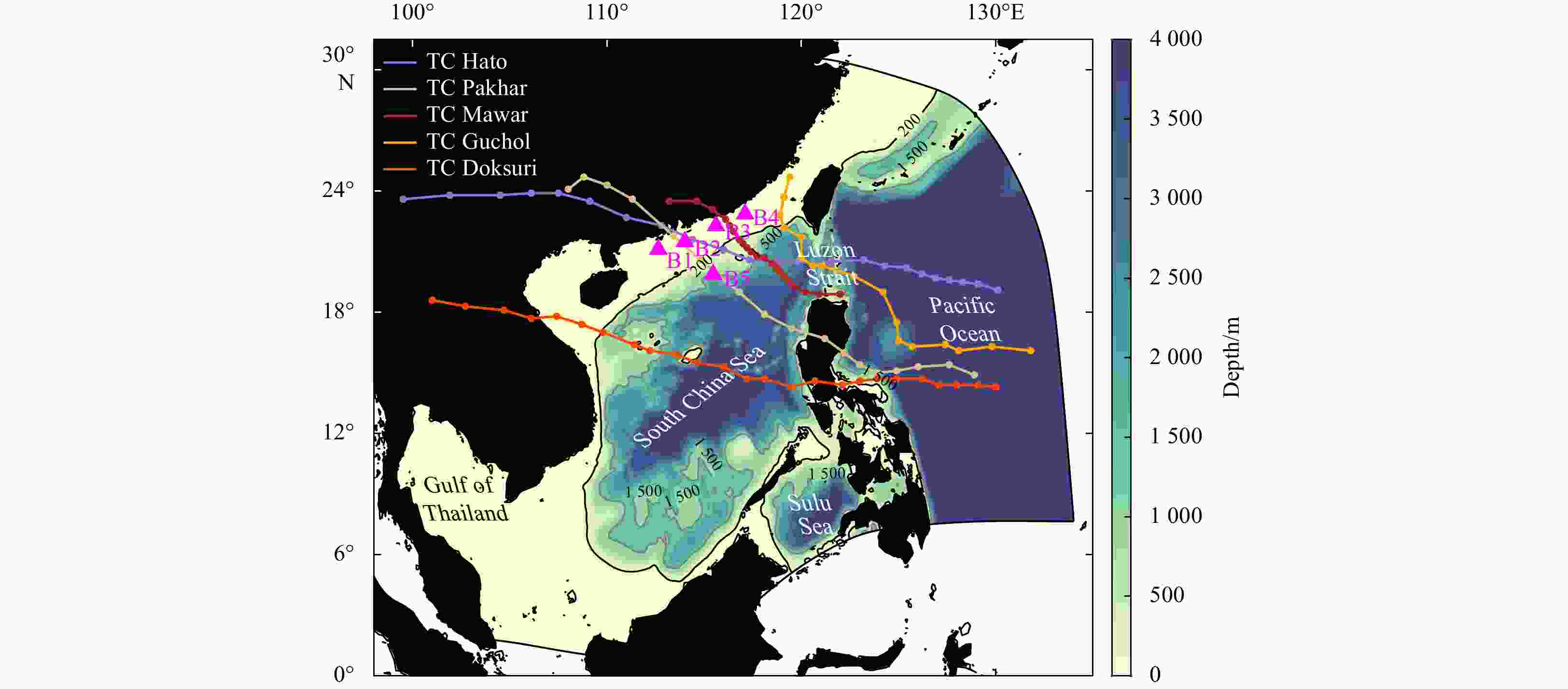
Figure 1. The study area, bathymetry (color fill), and tracks of five tropical cyclone (TCs) during the study period. The magenta triangles represent buoy positions.
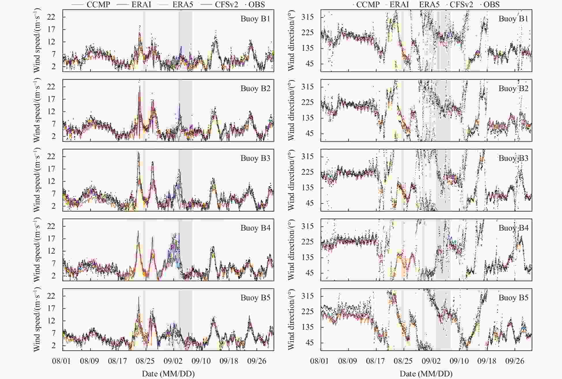
Figure 2. Time series of U10 (wind speed at 10 m height), wind direction between four wind data and corresponding buoy observations, with the time period from August 1 to September 30, 2017. The five periods of tropical cyclone (TC) occurrences are marked with a semi-transparent background color, from left to right: TC Hato, TC Pakhar, TC Mawar, TC Guchol, TC Doksuri. CCMP: Cross-Calibrated Multiplatform; ERAI: ECMWF Reanalysis-Interim; ERA5: ECMWF Reanalysis v5; CFSv2: NCEP Climate Forecast System Version 2; OBS: buoy observation.
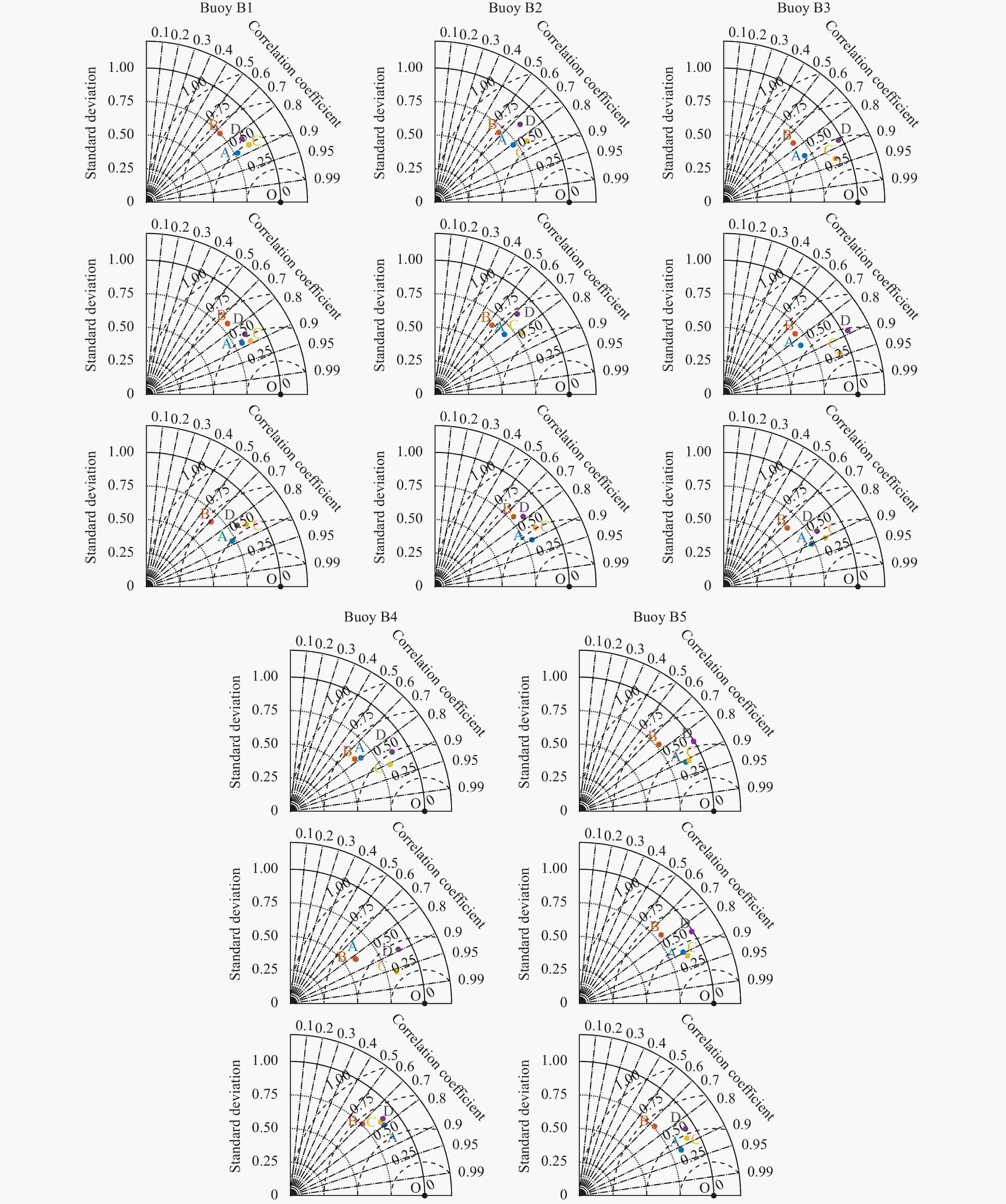
Figure 3. Taylor diagram of wind speeds at 10 m height (U10) comparison at five buoys. The three rows from top to bottom are the entire period of this study (from August 1 to September 30, 2017), tropical cyclone (TC)-only period, and TC-free period, respectively. The Points A, B, C, D, O in the Taylor diagram represent CCMP, ERAI, ERA5, CFSv2, and buoy observations, respectively. CCMP: Cross-Calibrated Multiplatform; ERAI: ECMWF Reanalysis-Interim; ERA5: ECMWF Reanalysis v5; CFSv2: NCEP Climate Forecast System Version 2.
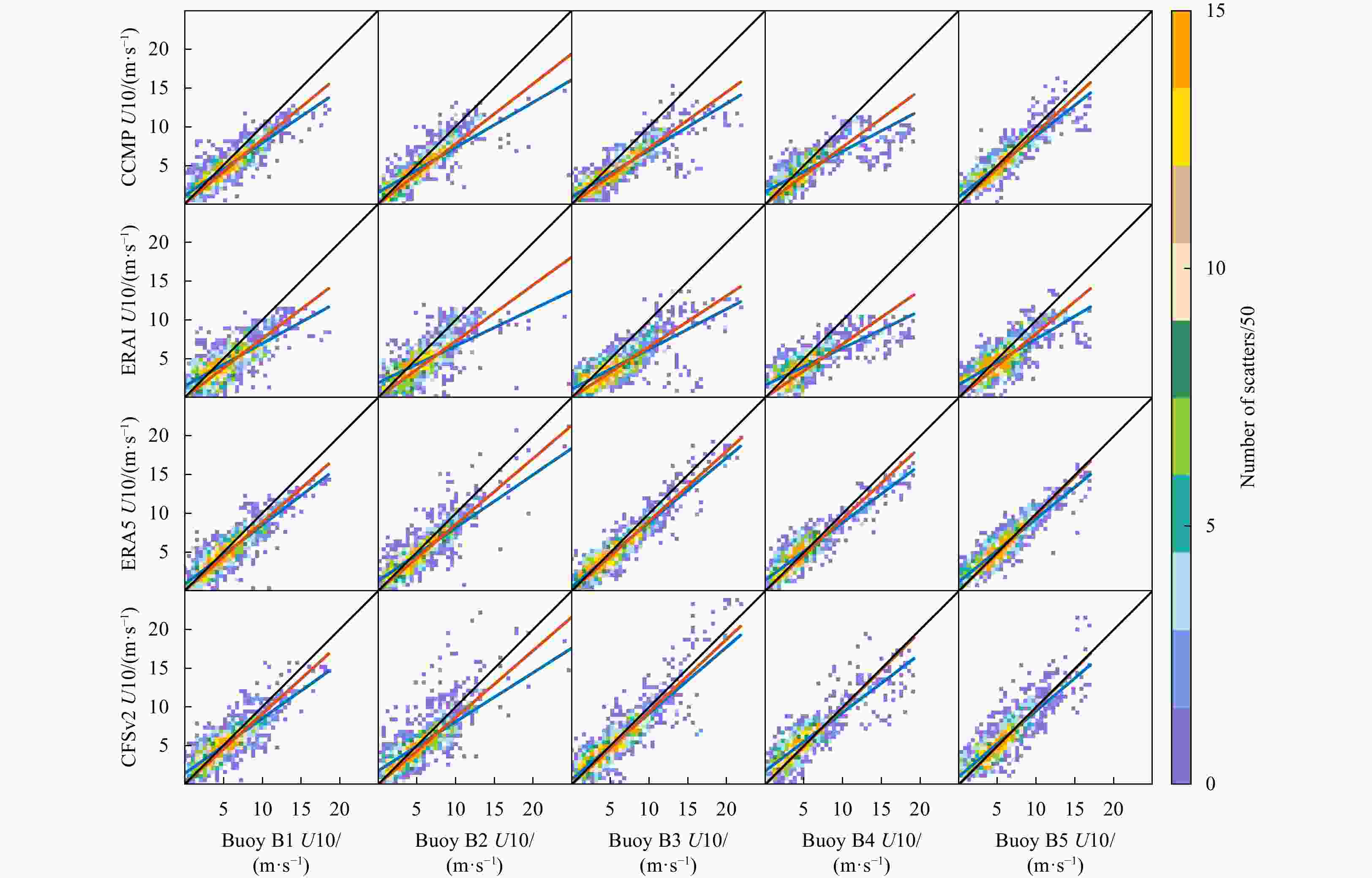
Figure 4. Scatter diagram of wind speeds at 10 m height (U10) obtained from four wind data and buoy observations between August 1 and September 30, 2017. The five columns from left to right represent five buoys. The x-axis represents U10 selected from the buoy observations, the y-axis represents U10 from the four wind products. The black lines represent for the perfect agreement between wind data and observations. The red lines and blue lines are fitted lines from different fitting formulas. CCMP: Cross-Calibrated Multiplatform; ERAI: ECMWF Reanalysis-Interim; ERA5: ECMWF Reanalysis v5; CFSv2: NCEP Climate Forecast System Version 2.
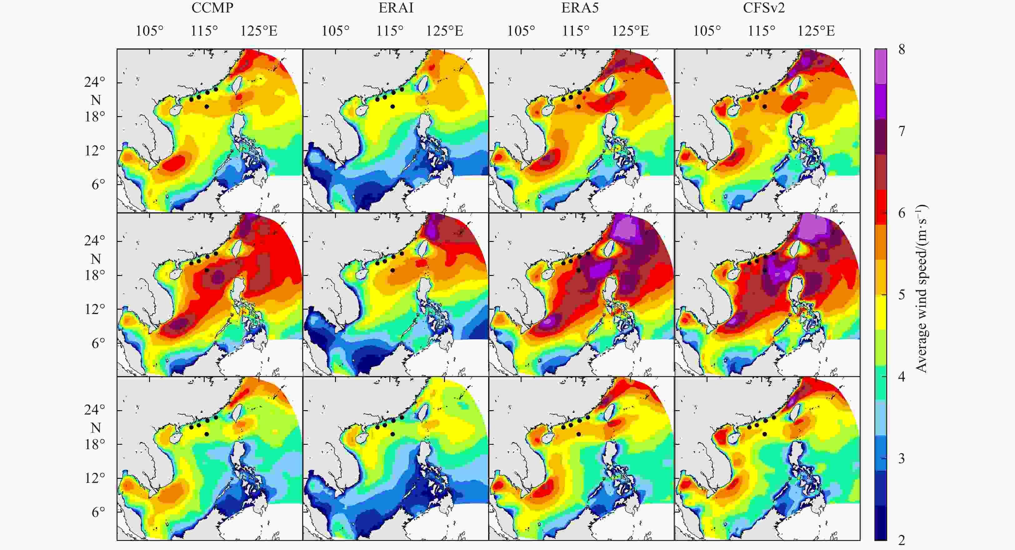
Figure 5. Magnitude of time-averaged wind speed in the study area. The four columns from left to right represent four wind data. The three rows from top to bottom represent the entire period, tropical cyclone (TC)-only period, and TC-free period. The black dots are the buoy positions. CCMP: Cross-Calibrated Multiplatform; ERAI: ECMWF Reanalysis-Interim; ERA5: ECMWF Reanalysis v5; CFSv2: NCEP Climate Forecast System Version 2.
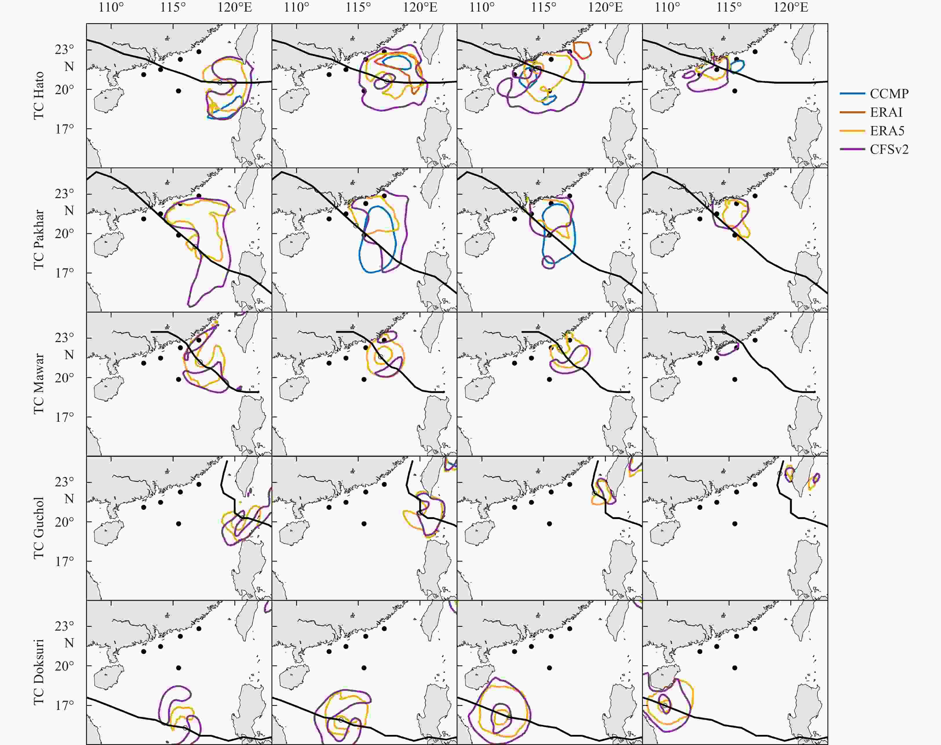
Figure 6. Contour distribution of the 99th percentile on wind speed during tropical cyclones (TCs). The five rows from top to bottom are five TC periods. The four columns are four snapshots during the TCs. The black lines are the TC tracks. The four colored contours represent four wind data. CCMP: Cross-Calibrated Multiplatform; ERAI: ECMWF Reanalysis-Interim; ERA5: ECMWF Reanalysis v5; CFSv2: NCEP Climate Forecast System Version 2.
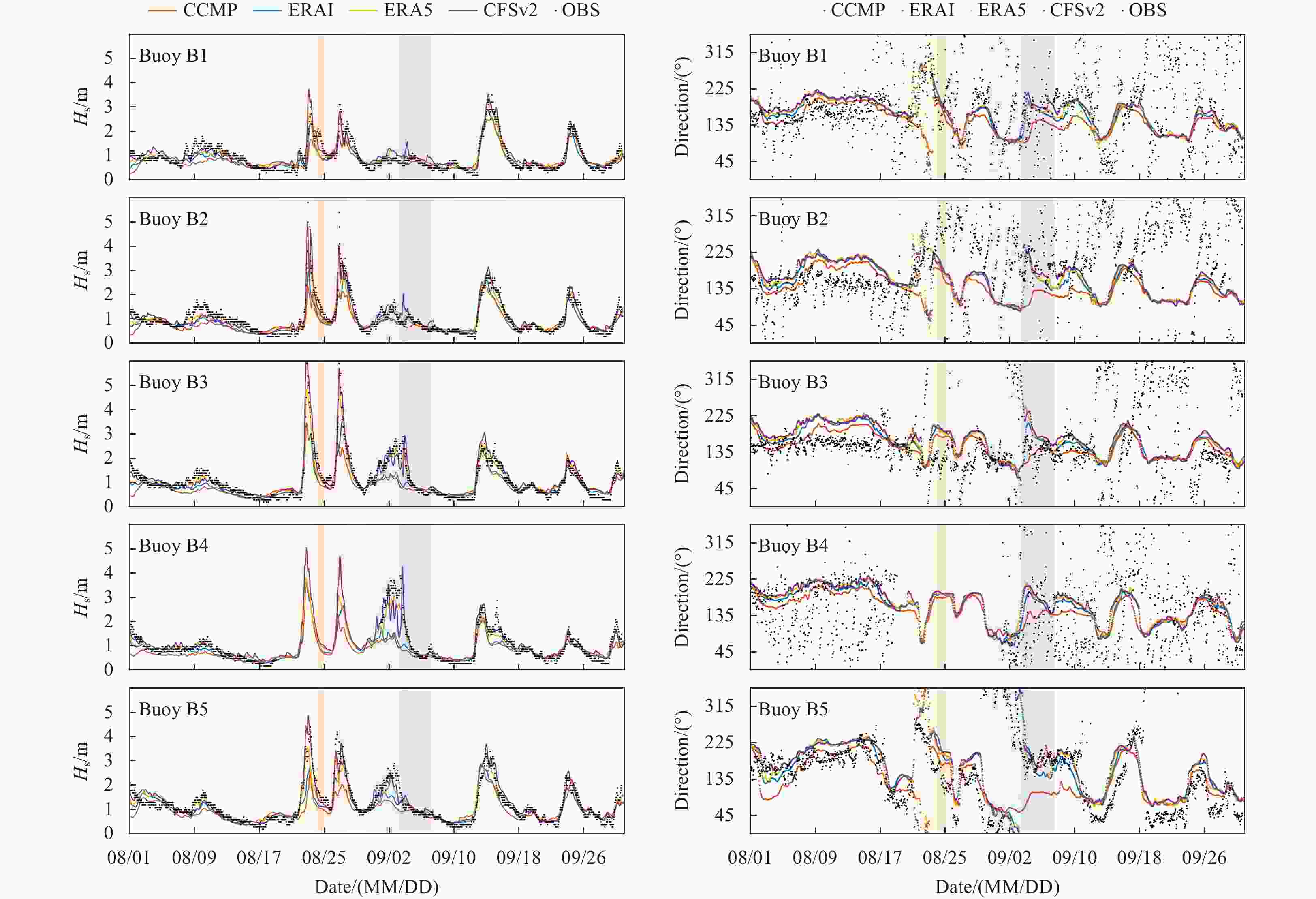
Figure 7. Time series comparison of Hs and wave direction obtained from corresponding wave hindcast and buoy observations. The five periods of tropical cyclone occurrences are marked with a semi-transparent background color, from left to right: TC Hato, TC Pakhar, TC Mawar, TC Guchol, TC Doksuri. Hs: significant wave height; CCMP: Cross-Calibrated Multiplatform; ERAI: ECMWF Reanalysis-Interim; ERA5: ECMWF Reanalysis v5; CFSv2: NCEP Climate Forecast System Version 2; OBS: buoy observation.
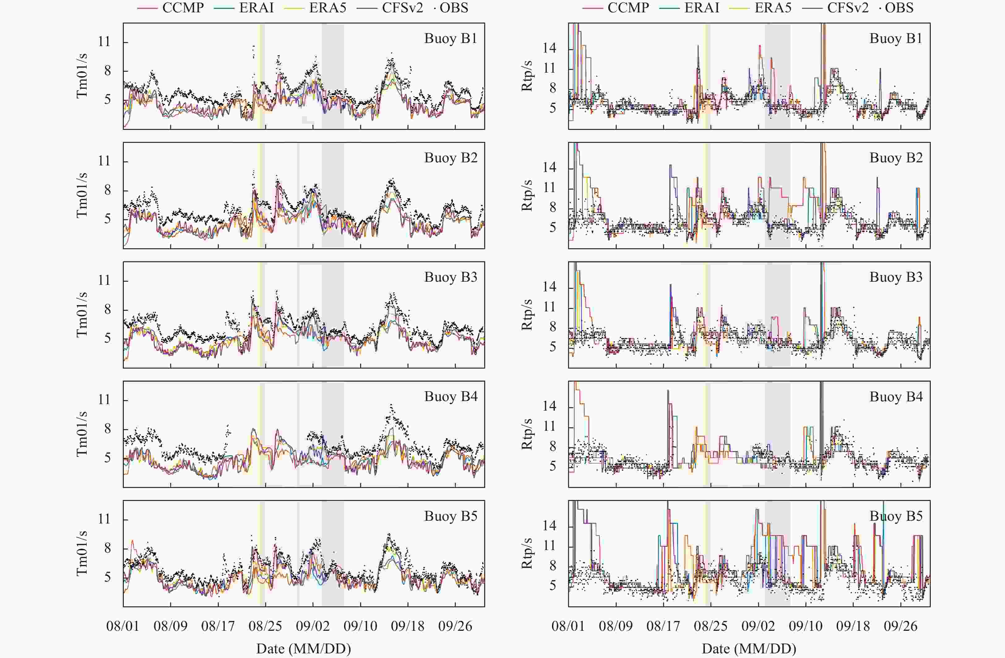
Figure 8. Time series comparison of mean absolute wave period (Tm01) and peak period of variance density spectrum (Rtp) obtained from corresponding wave hindcast and buoy observations. The five periods of tropical cyclone occurrences are marked with a semi-transparent background color. Tm01: mean absolute wave period; CCMP: Cross-Calibrated Multiplatform; ERAI: ECMWF Reanalysis-Interim; ERA5: ECMWF Reanalysis v5; CFSv2: NCEP Climate Forecast System Version 2; OBS: buoy observation.
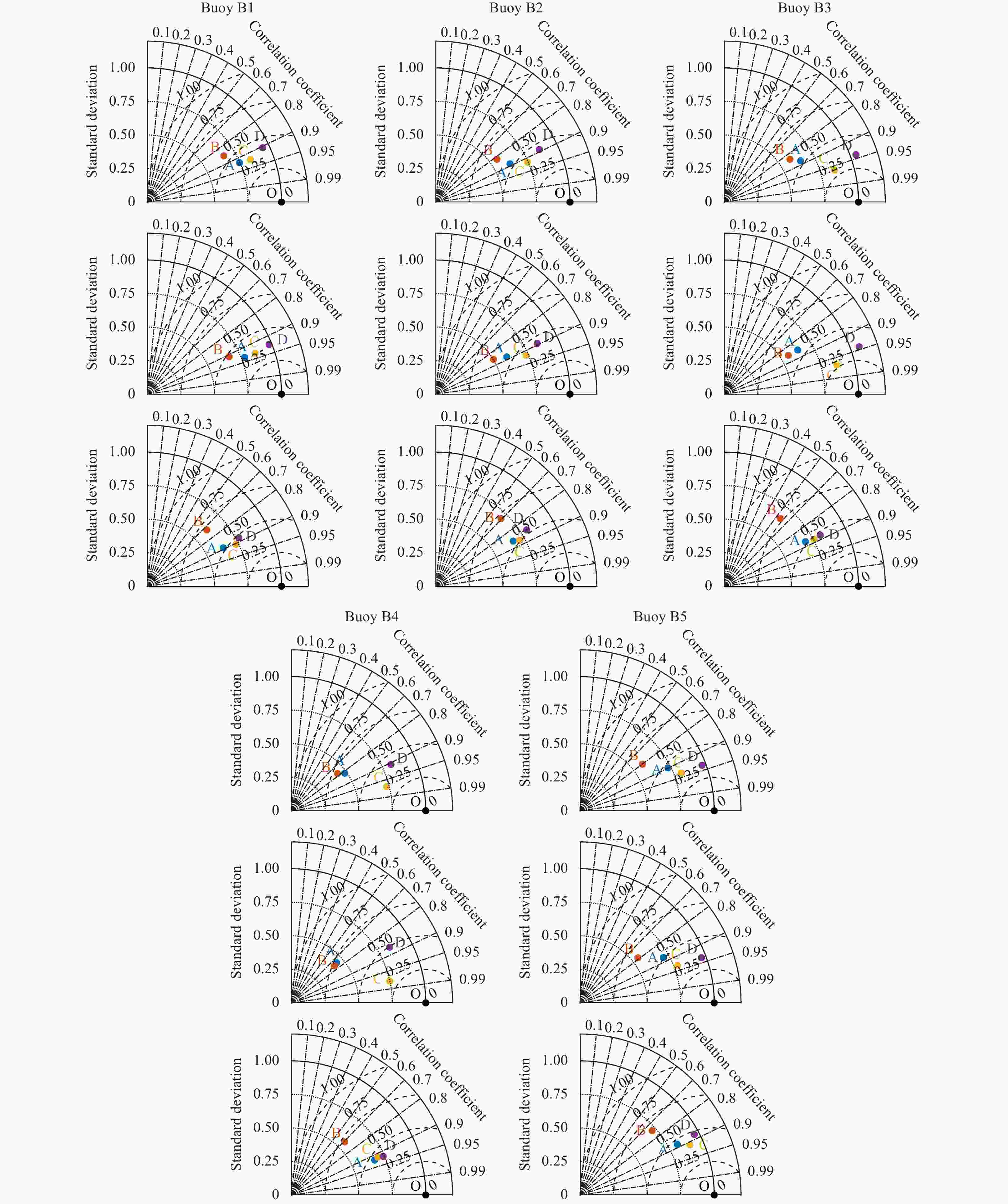
Figure 9. Taylor diagram of significant wave height comparison at five buoys. The three rows from top to bottom are the entire period, tropical cyclone (TC)-only period, and TC-period. The Points A, B, C, D, O in the Taylor diagram represent CCMP, ERAI, ERA5, CFSv2, and buoy observations, respectively. CCMP: Cross-Calibrated Multiplatform; ERAI: ECMWF Reanalysis-Interim; ERA5: ECMWF Reanalysis v5; CFSv2: NCEP Climate Forecast System Version 2.
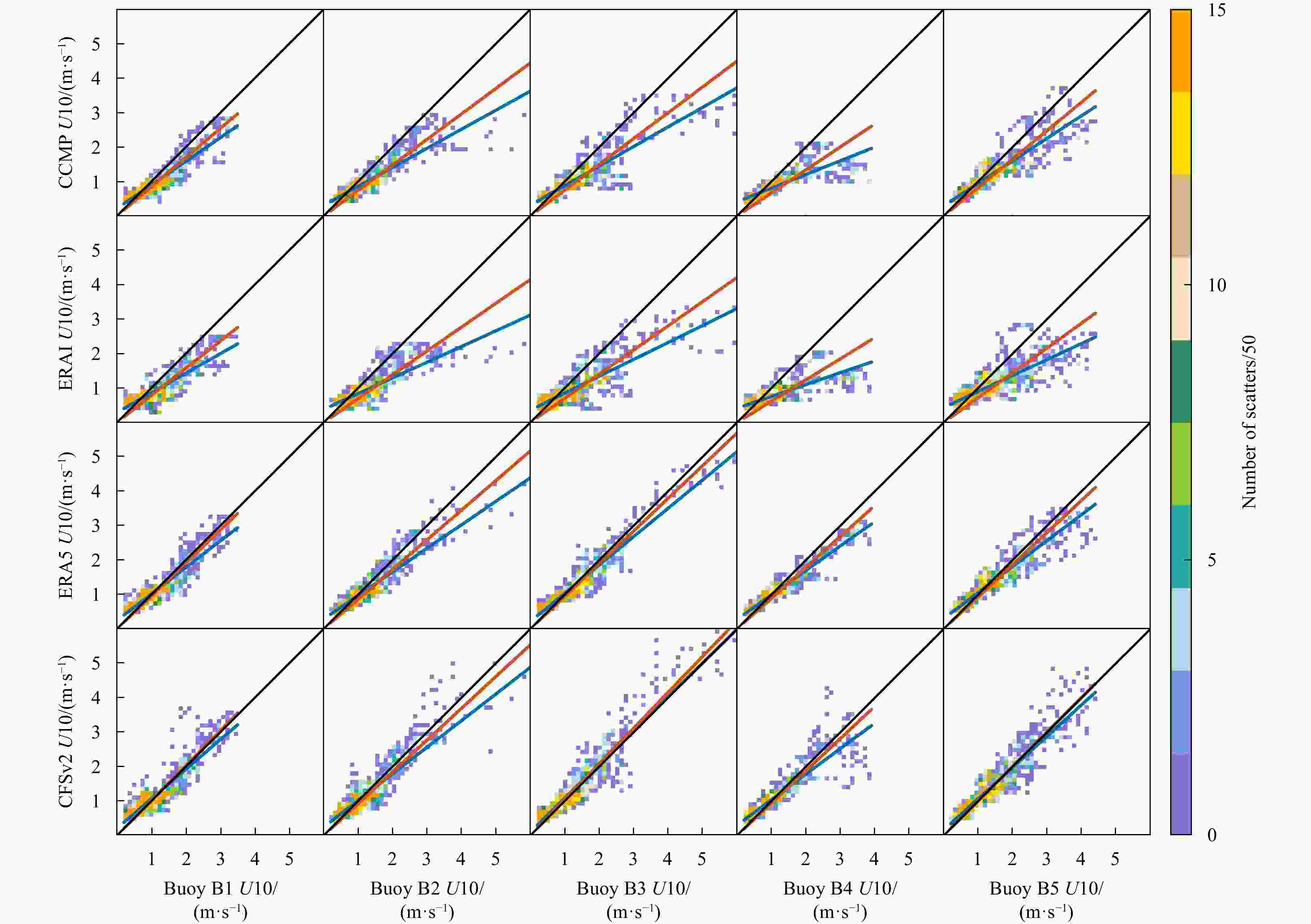
Figure 10. Scatter plot of Hs obtained from wave hindcasts and buoy observations over the entire period. The five columns from left to right represent five buoys. The x-axis represents Hs selected from buoy observations, the y-axis represents Hs from the four wind products. The black lines represent perfect agreement between wind data and observations. The red and blue lines are fitted lines from different fitting formulas. Hs: significant wave height; CCMP: Cross-Calibrated Multiplatform; ERAI: ECMWF Reanalysis-Interim; ERA5: ECMWF Reanalysis v5; CFSv2: NCEP Climate Forecast System Version 2.
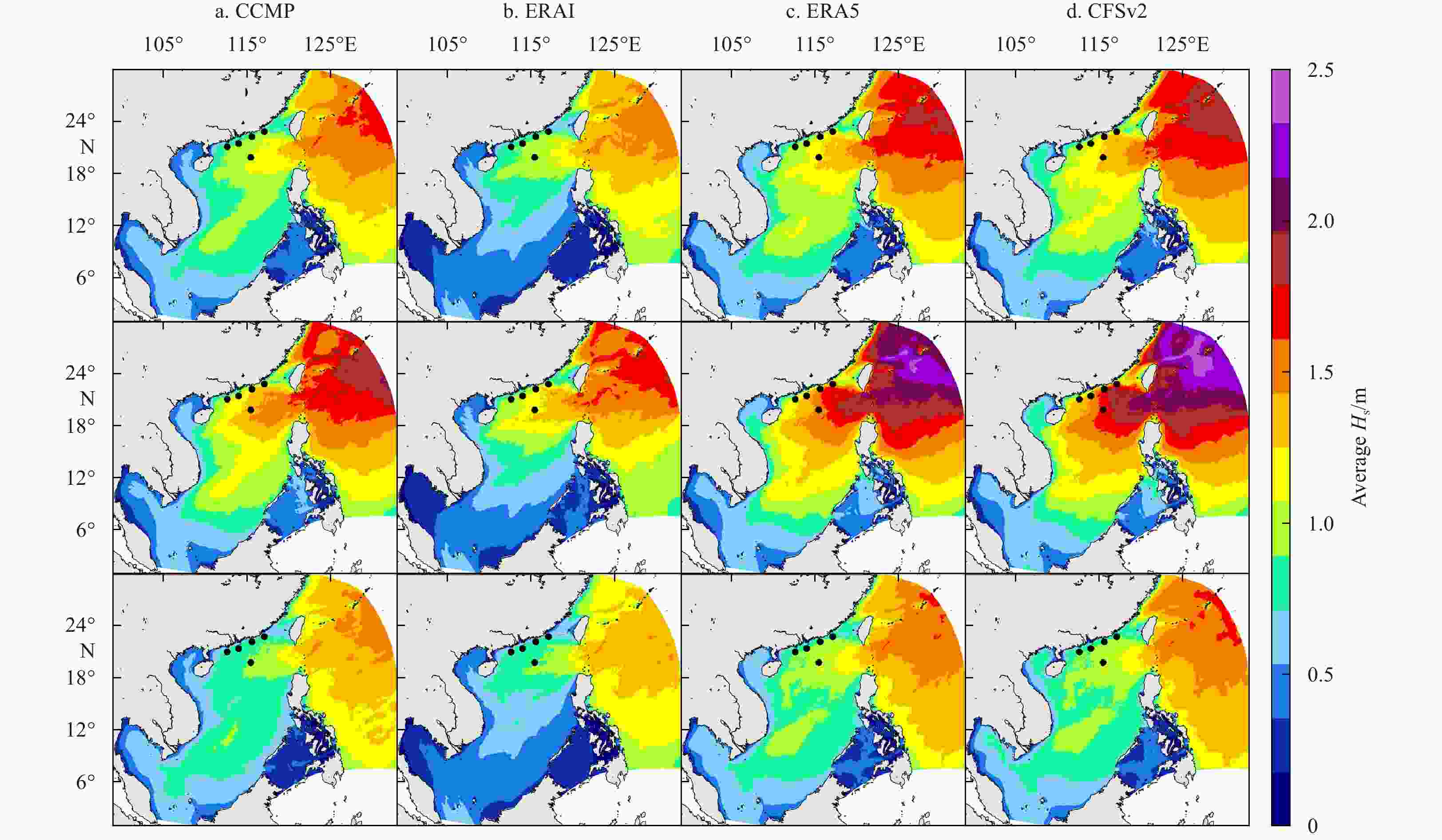
Figure 11. Magnitude of time-averaged Hs in the study area. The four columns from left to right represent four wind data. The three rows from top to bottom represent for entire period, tropical cyclone-only period, and tropical cyclone-free period. The black dots are the buoy positions. Hs: significant wave height; CCMP: Cross-Calibrated Multiplatform; ERAI: ECMWF Reanalysis-Interim; ERA5: ECMWF Reanalysis v5; CFSv2: NCEP Climate Forecast System Version 2.

Figure 12. Contour distribution of the 99th percentile of significant wave heights during tropical cyclone (TCs). The five rows from top to bottom are five TC periods. The four columns are four snapshots during the TCs. The black lines are the TC tracks. The four colored contours represent four wind data. CCMP: Cross-Calibrated Multiplatform; ERAI: ECMWF Reanalysis-Interim; ERA5: ECMWF Reanalysis v5; CFSv2: NCEP Climate Forecast System Version 2.
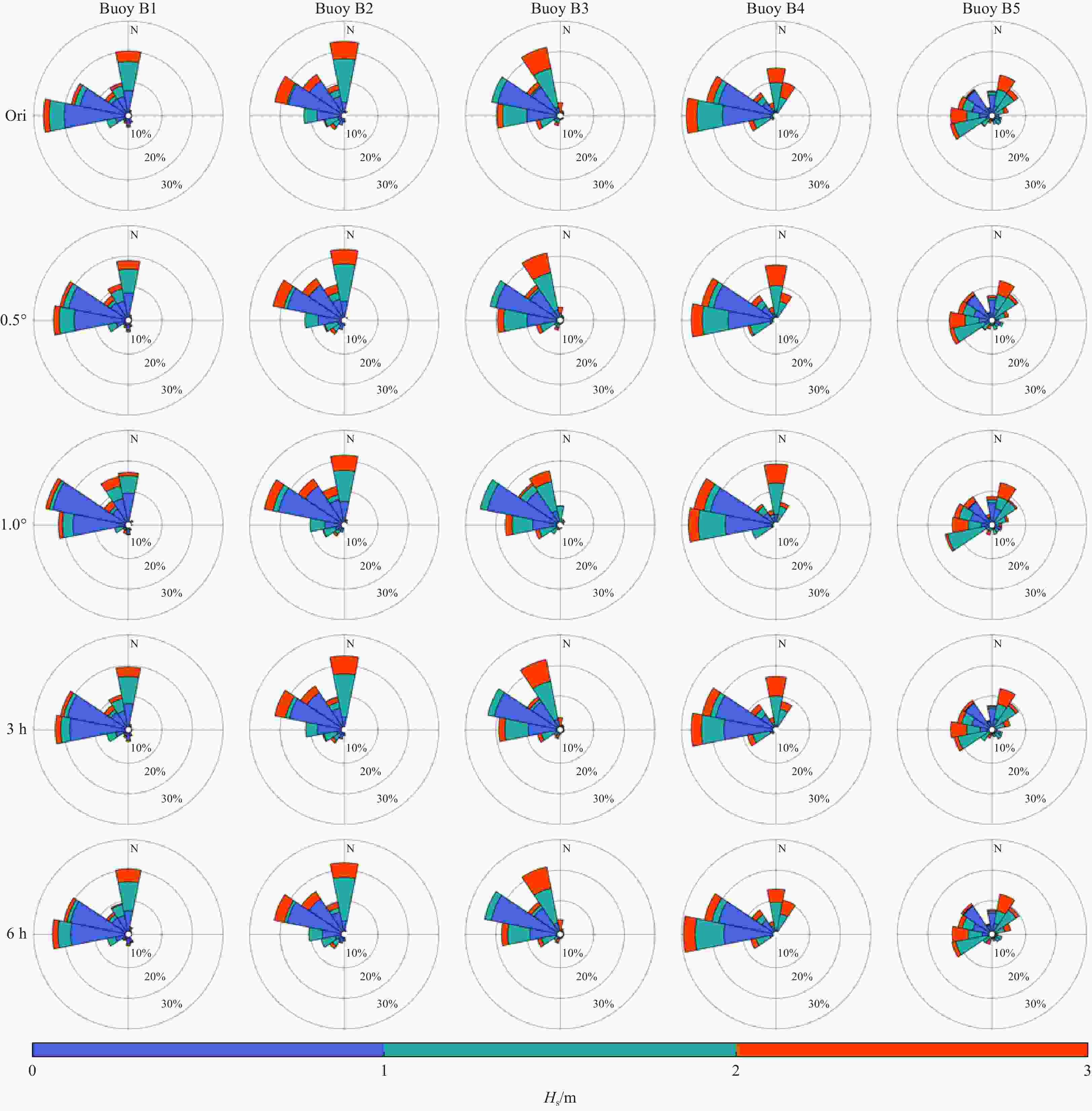
Figure 13. Waverose diagram of significant wave height (Hs) and wave direction obtained from experiments with different resolutions. The five rows from top to bottom correspond to the original results (Ori), spatial resolution of 0.5˚, spatial resolution of 1.0˚, temporal resolution of 3 h, and temporal resolution of 6 h, respectively. The five columns from left to right are at Buoys B1−B5. The three colors in each plot represent different ranges of Hs.
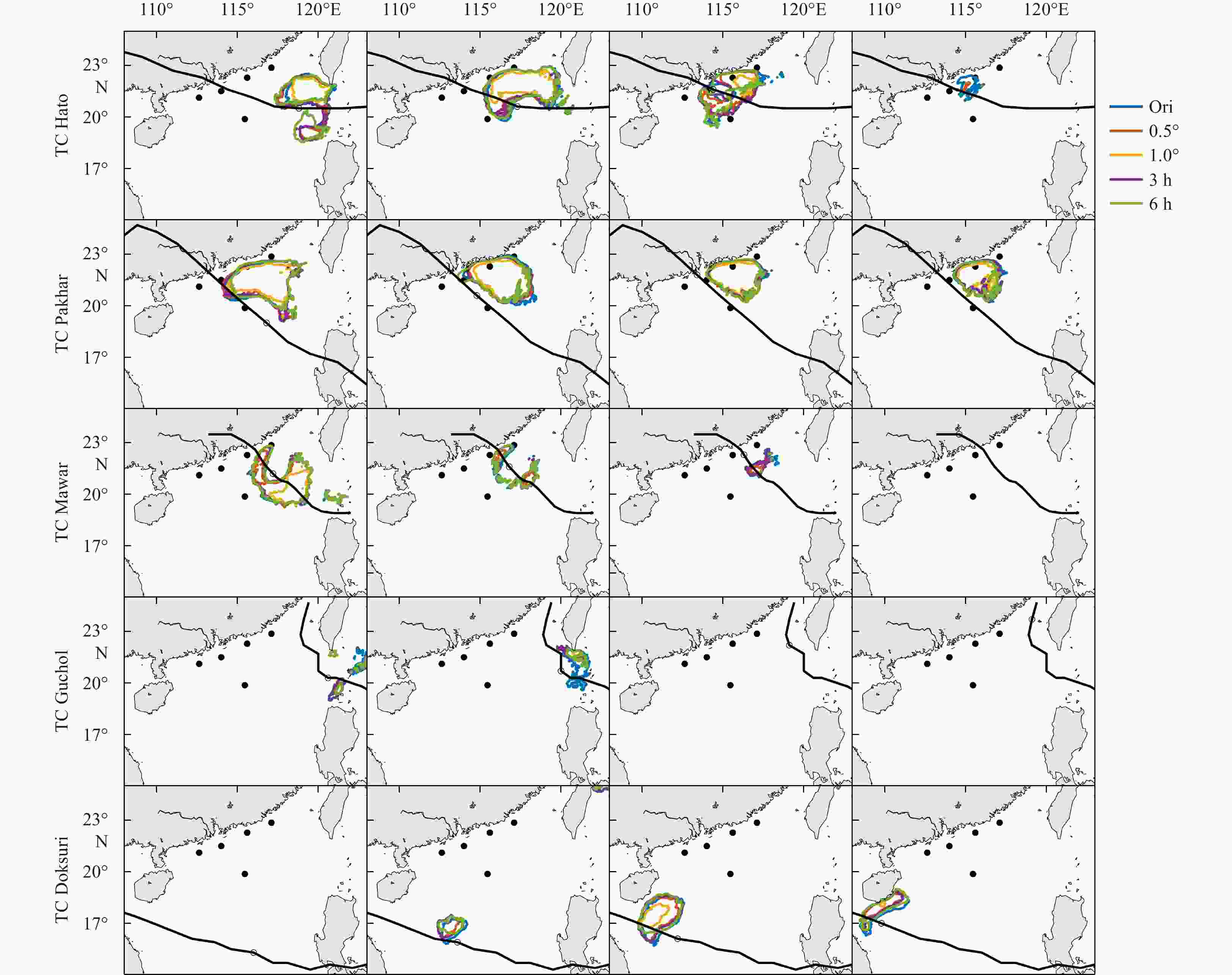
Figure 14. Contours represent the 99th percentile of significant wave height under different resolution experiments. The five rows from top to bottom are five tropical cyclone (TC) periods. The four columns are four snapshots during the TCs. The black lines are the TC tracks. CCMP: Cross-Calibrated Multiplatform; ERAI: ECMWF Reanalysis-Interim; ERA5: ECMWF Reanalysis v5; CFSv2: NCEP Climate Forecast System Version 2.
Table 1. Features of wind datasets
Data source Temporal coverage Temporal resolution/h Spatial resolution ERAI 1979−2019 3 0.25° ERA5 1979−2021 3 0.25° CFSv2 2011−present 1 0.125° CCMP 1987−present 6 0.25° Note: ERAI: ECMWF Reanalysis-Interim; ERA5: ECMWF Reanalysis v5; CFSv2: NCEP Climate Forecast System Version 2; CCMP: Cross-Calibrated Multiplatform.  下载: 导出CSV
Table 2. Features of buoys
Buoy Latitude Longitude Depth/m Number of Samples B1 21.12°N 112.63°E 50.43 1468 B2 21.50°N 114.00°E 54.02 1478 B3 22.28°N 115.60°E 49.17 1635 B4 22.87°N 117.10°E 40.60 1172 B5 19.87°N 115.46°E 1243.69 1472
下载: 导出CSV
Table 3. Average value (mean), maximum value of wind speed at 10 m height (U10) of the four wind data and corresponding hour when reaching the maximum value during each tropical cyclone period
Mean U10/(m·s−1) Maximum U10/(m·s−1) Occurrence of maximum U10/h Hato Pakhar Mawar Guchol Doksuri Hato Pakhar Mawar Guchol Doksuri Hato Pakhar Mawar Guchol Doksuri Buoy B1 6.67 7.20 3.38 3.26 6.25 18.60 15.20 7.40 11.10 16.60 92 64 113 33 104 CCMP 5.71 6.85 2.91 2.97 5.67 12.96 9.77 7.37 4.39 12.46 91 67 115 39 97 ERAI 4.69 7.30 2.29 1.60 5.70 10.05 9.97 4.71 2.97 11.67 97 64 31 42 109 ERA5 6.22 7.08 3.33 2.16 5.84 14.57 12.15 6.86 4.95 12.78 92 67 118 22 97 CFSv2 7.18 7.30 4.56 4.52 5.53 15.70 12.72 10.33 8.05 12.71 87 67 120 26 99 Buoy B2 7.41 8.11 4.09 2.94 5.54 43.40 19.30 11.10 10.60 13.90 87 69 79 39 96 CCMP 5.53 7.45 3.42 2.82 4.71 15.68 13.28 7.59 4.57 11.68 85 79 115 39 97 ERAI 4.92 7.92 2.80 1.66 5.00 12.09 11.59 5.19 3.43 10.96 97 79 43 39 97 ERA5 6.69 8.02 4.13 3.15 5.22 21.42 15.17 9.32 5.51 12.16 89 74 112 29 92 CFSv2 6.93 8.35 4.13 4.69 5.17 22.39 16.87 15.34 6.83 12.47 91 76 109 42 91 Buoy B3 6.94 8.22 7.25 2.74 5.26 21.80 20.00 16.90 5.40 13.40 83 71 107 43 80 CCMP 5.33 6.94 4.56 2.09 4.21 15.52 13.25 7.00 3.59 9.82 91 73 121 45 91 ERAI 5.16 6.81 4.16 1.23 3.98 13.91 12.25 7.65 2.12 9.45 91 76 85 45 82 ERA5 6.37 8.06 6.75 2.44 4.83 19.68 18.11 14.94 5.00 11.41 83 68 110 41 82 CFSv2 7.48 8.39 6.54 2.49 5.17 24.04 20.01 15.98 4.79 13.23 80 74 111 45 90 Buoy B4 NaN NaN 12.96 3.03 5.56 NaN NaN 19.20 5.60 13.80 NaN NaN 81 40 82 CCMP 5.54 5.74 7.30 2.45 4.56 15.29 11.31 11.13 4.80 11.32 79 73 43 45 85 ERAI 5.72 5.70 6.92 1.52 4.37 15.43 11.61 10.57 2.55 10.62 82 61 82 42 85 ERA5 5.80 6.14 10.46 3.07 5.06 15.32 13.11 16.58 6.50 11.61 78 67 80 41 80 CFSv2 6.89 6.65 10.78 2.74 5.75 20.22 17.97 19.33 6.18 14.15 80 70 105 45 85 Buoy B5 6.42 8.59 6.53 3.84 6.00 16.80 17.00 10.30 6.20 13.80 81 76 74 18 94 CCMP 6.10 8.60 6.78 4.11 5.48 13.83 16.30 8.81 5.13 11.56 91 73 25 21 97 ERAI 5.54 7.91 4.64 1.90 6.10 14.00 11.15 6.69 3.77 11.29 88 76 31 39 85 ERA5 6.60 8.50 7.07 4.52 5.70 16.38 14.52 10.04 7.16 12.47 82 58 72 40 90 CFSv2 7.35 8.36 7.71 4.99 5.53 21.72 14.59 11.20 7.58 12.92 83 73 69 18 87 Note: CCMP: Cross-Calibrated Multiplatform; ERAI: ECMWF Reanalysis-Interim; ERA5: ECMWF Reanalysis v5; CFSv2: NCEP Climate Forecast System Version 2. NaN indicates data unavailability.
下载: 导出CSV
Table 4. Statistical parameters for RMSE, r2, BIAS, SI and fitting coefficients (b and c) of wind speed at 10 m height (U10) based on four wind data and buoy observations during entire period, tropical cyclone (TC)-only period, and TC-free period
Entire period TC-only period TC-free period RMSE r2 BIAS SI b c RMSE r2 BIAS SI b c RMSE r2 BIAS SI b c Buoy B1 CCMP 0.49 0.88 0.68 0.09 0.68 0.83 0.48 0.88 0.62 0.09 0.71 0.84 0.50 0.88 0.71 0.09 0.64 0.83 ERAI 0.68 0.73 0.99 0.12 0.55 0.76 0.66 0.75 1.12 0.12 0.60 0.74 0.71 0.71 0.91 0.12 0.48 0.77 ERA5 0.49 0.87 0.46 0.09 0.76 0.88 0.46 0.89 0.39 0.08 0.78 0.89 0.53 0.85 0.50 0.08 0.75 0.88 CFSv2 0.55 0.83 0.19 0.10 0.71 0.91 0.52 0.85 −0.27 0.09 0.73 0.96 0.56 0.83 0.47 0.10 0.68 0.87 Buoy B2 CCMP 0.60 0.81 0.82 0.11 0.58 0.78 0.66 0.76 0.95 0.11 0.52 0.72 0.45 0.90 0.74 0.12 0.72 0.84 ERAI 0.74 0.67 0.97 0.13 0.47 0.73 0.77 0.64 1.27 0.13 0.43 0.65 0.67 0.75 0.79 0.15 0.59 0.80 ERA5 0.55 0.83 0.43 0.10 0.69 0.86 0.58 0.82 0.26 0.10 0.65 0.84 0.51 0.86 0.53 0.11 0.75 0.87 CFSv2 0.69 0.74 0.26 0.12 0.63 0.86 0.71 0.71 0.02 0.12 0.61 0.85 0.62 0.78 0.40 0.14 0.66 0.88 Buoy B3 CCMP 0.53 0.87 1.28 0.09 0.60 0.72 0.56 0.84 1.57 0.09 0.57 0.69 0.47 0.90 1.10 0.11 0.66 0.76 ERAI 0.65 0.76 1.61 0.12 0.52 0.66 0.65 0.76 1.89 0.10 0.53 0.65 0.68 0.73 1.44 0.13 0.47 0.67 ERA5 0.37 0.93 0.39 0.07 0.83 0.90 0.33 0.94 0.43 0.05 0.87 0.91 0.44 0.90 0.37 0.07 0.76 0.89 CFSv2 0.49 0.88 0.17 0.09 0.86 0.94 0.48 0.89 0.07 0.08 0.92 0.97 0.51 0.86 0.23 0.10 0.69 0.90 Buoy B4 CCMP 0.62 0.80 0.86 0.12 0.52 0.74 0.61 0.83 2.12 0.09 0.49 0.62 0.61 0.80 0.39 0.14 0.70 0.87 ERAI 0.65 0.78 1.09 0.13 0.48 0.69 0.61 0.82 2.36 0.09 0.48 0.59 0.71 0.71 0.62 0.14 0.54 0.80 ERA5 0.43 0.91 −0.08 0.08 0.74 0.93 0.32 0.96 0.59 0.05 0.79 0.87 0.64 0.77 −0.34 0.07 0.67 1.00 CFSv2 0.50 0.86 −0.48 0.10 0.76 0.99 0.45 0.89 0.15 0.06 0.80 0.91 0.65 0.77 −0.72 0.10 0.69 1.07 Buoy B5 CCMP 0.42 0.91 0.21 0.08 0.79 0.92 0.44 0.90 0.06 0.07 0.77 0.94 0.42 0.91 0.29 0.09 0.76 0.91 ERAI 0.64 0.76 0.57 0.12 0.59 0.83 0.64 0.77 0.92 0.10 0.61 0.80 0.68 0.73 0.37 0.13 0.56 0.86 ERA5 0.42 0.91 −0.18 0.08 0.82 0.99 0.41 0.91 −0.21 0.06 0.80 0.98 0.47 0.88 −0.17 0.08 0.80 1.00 CFSv2 0.54 0.85 −0.20 0.10 0.85 1.00 0.56 0.84 −0.52 0.09 0.84 1.02 0.54 0.85 −0.01 0.11 0.79 0.97 Note: RMSE: root mean square error; r2: correlation coefficient; SI: scatter index; CCMP: Cross-Calibrated Multiplatform; ERAI: ECMWF Reanalysis-Interim; ERA5: ECMWF Reanalysis v5; CFSv2: NCEP Climate Forecast System Version 2.
下载: 导出CSV
Table 5. The average value of significant wave height (Hs) (mean Hs), maximum value of Hs from wave hindcasts, and the corresponding time when reaching the maximum values during tropical cyclones for buoy observations and four wind data
Mean Hs/m Maximum Hs/m Occurence of maximum Hs/h Hato Pakhar Mawar Guchol Doksuri Hato Pakhar Mawar Guchol Doksuri Hato Pakhar Mawar Guchol Doksuri Buoy B1 1.05 1.60 0.70 0.60 1.39 3.20 3.10 1.00 0.80 3.50 94 70 60 1 113 CCMP 0.92 1.22 0.77 0.67 1.31 2.32 1.95 0.97 0.79 2.87 93 91 117 1 100 ERAI 0.84 1.21 0.74 0.61 1.27 1.67 1.88 0.87 0.75 2.54 97 68 75 1 110 ERA5 1.07 1.35 0.90 0.72 1.43 2.72 2.58 1.22 0.78 3.30 90 70 71 1 105 CFSv2 1.27 1.47 0.99 0.86 1.49 3.74 2.80 1.56 1.03 3.54 88 71 121 27 102 Buoy B2 1.44 1.96 1.03 0.64 1.36 8.50 5.40 1.80 0.90 3.00 87 69 82 3 99 CCMP 1.01 1.46 0.89 0.65 1.23 2.98 2.93 1.12 0.74 2.61 86 83 59 1 98 ERAI 0.96 1.36 0.86 0.60 1.22 2.34 2.29 1.05 0.72 2.34 86 65 70 1 87 ERA5 1.27 1.62 1.09 0.68 1.39 4.21 3.49 1.63 0.74 2.86 84 68 74 1 103 CFSv2 1.43 1.78 1.19 0.81 1.47 4.97 4.04 2.04 0.95 3.16 83 68 109 42 102 Buoy B3 1.47 2.13 1.85 0.61 1.22 6.10 6.00 2.90 0.80 2.60 82 70 106 36 121 CCMP 1.19 1.65 1.07 0.70 1.16 3.47 3.55 1.37 0.74 2.34 81 79 70 1 88 ERAI 1.27 1.42 1.07 0.65 1.15 3.36 2.61 1.43 0.71 2.31 82 64 87 1 84 ERA5 1.51 1.95 1.61 0.75 1.33 5.00 5.00 2.71 0.84 2.65 83 69 110 42 82 CFSv2 1.79 2.13 1.70 0.76 1.47 6.66 5.70 2.94 0.84 3.07 81 68 113 42 91 Buoy B4 NaN NaN 2.86 0.65 1.25 NaN NaN 3.90 1.10 2.90 NaN NaN 99 36 128 CCMP 1.24 1.38 1.25 0.64 1.02 3.64 2.68 1.77 0.67 2.16 80 80 44 24 86 ERAI 1.29 1.20 1.15 0.56 1.02 3.65 2.32 1.55 0.58 2.08 81 64 83 29 83 ERA5 1.38 1.53 2.04 0.71 1.16 3.82 3.09 3.14 0.84 2.28 80 67 82 42 81 CFSv2 1.62 1.78 2.14 0.70 1.33 5.07 4.70 4.29 0.79 2.75 80 71 106 45 88 Buoy B5 1.60 2.19 1.80 0.81 1.47 4.40 4.20 2.90 0.90 3.50 92 62 82 8 93 CCMP 1.21 1.83 1.34 0.84 1.40 2.77 3.76 1.72 0.90 2.81 91 75 52 1 84 ERAI 1.05 1.35 1.13 0.75 1.44 2.60 2.03 1.40 0.88 2.87 91 78 55 1 82 ERA5 1.48 1.84 1.54 0.93 1.61 3.54 3.31 2.27 1.01 3.23 84 59 73 18 95 CFSv2 1.73 1.94 1.69 0.94 1.69 4.88 3.42 2.47 1.10 3.71 86 59 71 19 96 Note: CCMP: Cross-Calibrated Multiplatform; ERAI: ECMWF Reanalysis-Interim; ERA5: ECMWF Reanalysis v5; CFSv2: NCEP Climate Forecast System Version 2. NaN indicates data unavailability.
下载: 导出CSV
Table 6. Statistical parameters of RMSE, r2, BIAS, SI and fitting coefficients (b and c) for Hs obtained from four wind data and buoy observations during entire period, tropical cyclone (TC)-only period, and TC-free period
Entire period TC-only period TC-free period RMSE r2 BIAS SI b c RMSE r2 BIAS SI b c RMSE r2 BIAS SI b c Buoy B1 CCMP 0.43 0.92 0.09 0.45 0.69 0.85 0.39 0.94 0.08 0.35 0.72 0.86 0.52 0.89 0.09 0.44 0.57 0.83 ERAI 0.55 0.86 0.12 0.58 0.57 0.79 0.48 0.91 0.13 0.44 0.61 0.80 0.70 0.73 0.12 0.54 0.44 0.78 ERA5 0.39 0.92 −0.03 0.41 0.77 0.96 0.36 0.93 −0.04 0.33 0.80 0.96 0.46 0.90 −0.03 0.41 0.66 0.95 CFSv2 0.43 0.90 −0.07 0.45 0.86 1.02 0.38 0.93 −0.16 0.35 0.91 1.07 0.48 0.88 −0.03 0.43 0.68 0.96 Buoy B2 CCMP 0.53 0.89 0.17 0.50 0.55 0.74 0.55 0.89 0.27 0.40 0.53 0.70 0.54 0.86 0.12 0.60 0.58 0.81 ERAI 0.63 0.82 0.19 0.60 0.46 0.69 0.63 0.86 0.32 0.46 0.43 0.64 0.72 0.69 0.13 0.69 0.49 0.78 ERA5 0.43 0.92 0.04 0.41 0.68 0.86 0.44 0.92 0.09 0.32 0.67 0.84 0.51 0.88 0.03 0.48 0.63 0.90 CFSv2 0.45 0.89 0.00 0.43 0.77 0.92 0.45 0.89 −0.04 0.33 0.76 0.93 0.53 0.85 0.01 0.49 0.68 0.91 Buoy B3 CCMP 0.53 0.88 0.17 0.48 0.57 0.75 0.56 0.86 0.32 0.36 0.55 0.70 0.52 0.88 0.10 0.61 0.61 0.86 ERAI 0.60 0.84 0.20 0.55 0.49 0.70 0.60 0.86 0.36 0.39 0.48 0.66 0.77 0.64 0.13 0.65 0.42 0.79 ERA5 0.30 0.96 −0.02 0.27 0.82 0.95 0.27 0.97 0.02 0.18 0.84 0.93 0.48 0.89 −0.04 0.30 0.67 0.98 CFSv2 0.35 0.94 −0.08 0.32 0.98 1.04 0.35 0.94 −0.15 0.23 1.01 1.06 0.47 0.88 −0.05 0.39 0.72 0.99 Buoy B4 CCMP 0.66 0.82 0.19 0.67 0.40 0.67 0.73 0.75 0.55 0.47 0.34 0.54 0.46 0.92 0.11 0.84 0.62 0.87 ERAI 0.71 0.78 0.24 0.72 0.34 0.62 0.73 0.76 0.59 0.47 0.32 0.52 0.72 0.71 0.16 0.85 0.40 0.78 ERA5 0.34 0.97 0.01 0.35 0.71 0.90 0.31 0.98 0.17 0.20 0.73 0.84 0.45 0.92 −0.03 0.36 0.65 0.99 CFSv2 0.43 0.91 −0.04 0.44 0.74 0.94 0.49 0.87 0.06 0.32 0.73 0.89 0.43 0.92 −0.06 0.57 0.68 1.02 Buoy B5 CCMP 0.47 0.90 0.13 0.39 0.66 0.83 0.51 0.88 0.27 0.31 0.62 0.78 0.47 0.89 0.06 0.50 0.73 0.91 ERAI 0.64 0.80 0.21 0.53 0.46 0.72 0.66 0.79 0.45 0.40 0.43 0.66 0.67 0.75 0.10 0.66 0.54 0.84 ERA5 0.37 0.94 −0.01 0.31 0.75 0.93 0.39 0.93 0.11 0.24 0.73 0.89 0.42 0.91 −0.06 0.39 0.82 1.02 CFSv2 0.35 0.94 −0.05 0.29 0.91 1.00 0.35 0.94 −0.04 0.21 0.90 1.00 0.48 0.88 −0.05 0.35 0.85 1.01 Note: Hs: significant wave height; RMSE: root mean square error; r2: correlation coefficient; SI: scatter index; CCMP: Cross-Calibrated Multiplatform; ERAI: ECMWF Reanalysis-Interim; ERA5: ECMWF Reanalysis v5; CFSv2: NCEP Climate Forecast System Version 2.
下载: 导出CSV
-
Atlas R, Hoffman R N, Bloom S C, et al. 1996. A multiyear global surface wind velocity dataset using SSM/I wind observations. Bulletin of the American Meteorological Society, 77(5): 869–882. doi: 10.1175/1520-0477(1996)077<0869:AMGSWV>2.0.CO;2 Atlas R, Hoffman R N, Ardizzone J, et al. 2011. A cross-calibrated, multiplatform ocean surface wind velocity product for meteorological and oceanographic applications. Bulletin of the American Meteorological Society, 92(2): 157–174. doi: 10.1175/2010BAMS2946.1 Battjes J A, Janssen J P F M. 1978. Energy loss and set-up due to breaking of random waves. In: Proceedings of the 16th International Conference on Coastal Engineering. Hamburg, Germany: American Society of Civil Engineers, 569–587 Becerra D, Quezada M, Díaz H. 2022. A deep water and nearshore wave height calibration of the ECOWAVES hindcasting database. Latin American Journal of Aquatic Research, 50(4): 573–595. doi: 10.3856/vol50-issue4-fulltext-2811 Booij N, Ris R C, Holthuijsen L H. 1999. A third-generation wave model for coastal regions: 1. Model description and validation. Journal of Geophysical Research: Oceans, 104(C4): 7649–7666. doi: 10.1029/98JC02622 Bourassa M A, Legler D M, O’Brien J J, et al. 2003. SeaWinds validation with research vessels. Journal of Geophysical Research: Oceans, 108(C2): 3019 Carvalho D, Rocha A, Gómez-Gesteira M, et al. 2014. Comparison of reanalyzed, analyzed, satellite-retrieved and NWP modelled winds with buoy data along the Iberian Peninsula coast. Remote Sensing of Environment, 152: 480–492. doi: 10.1016/j.rse.2014.07.017 Cavaleri L, Rizzoli P M. 1981. Wind wave prediction in shallow water: Theory and applications. Journal of Geophysical Research: Oceans, 86(C11): 10961–10973. doi: 10.1029/JC086iC11p10961 Chalikov D. 2018. Numerical modeling of surface wave development under the action of wind. Ocean Science, 14(3): 453–470. doi: 10.5194/os-14-453-2018 Chauvin F, Douville H, Ribes A. 2017. Atlantic tropical cyclones water budget in observations and CNRM-CM5 model. Climate Dynamics, 49(11): 4009–4021 Chelton D B, Freilich M H. 2005. Scatterometer-based assessment of 10-m wind analyses from the operational ECMWF and NCEP numerical weather prediction models. Monthly Weather Review, 133(2): 409–429. doi: 10.1175/MWR-2861.1 Chen Weibo, Chen Hongey, Hsiao Shihchun, et al. 2019. Wind forcing effect on hindcasting of typhoon-driven extreme waves. Ocean Engineering, 188: 106260. doi: 10.1016/j.oceaneng.2019.106260 Dee D P, Uppala S M, Simmons A J, et al. 2011. The ERA-Interim reanalysis: Configuration and performance of the data assimilation system. Quarterly Journal of the Royal Meteorological Society, 137(656): 553–597. doi: 10.1002/qj.828 Gualtieri G. 2021. Reliability of ERA5 reanalysis data for wind resource assessment: A comparison against tall towers. Energies, 14(14): 4169. doi: 10.3390/en14144169 Hasselmann K, Barnett T, Bouws E, et al. 1973. Measurements of wind-wave growth and swell decay during the Joint North Sea Wave Project (JONSWAP). In: Ergänzungsheft zur Deutschen Hydrographischen Zeitschrift. Hamburg: Deutches Hydrographisches Institut, 8: 1–95 Hasselmann S, Hasselmann K, Allender J H, et al. 1985. Computations and parameterizations of the nonlinear energy transfer in a gravity-wave spectrum. Part II: Parameterizations of the nonlinear energy transfer for application in wave models. Journal of Physical Oceanography, 15(11): 1378–1391. doi: 10.1175/1520-0485(1985)015<1378:CAPOTN>2.0.CO;2 Hawkins S, Eager D, Harrison G P. 2011. Characterising the reliability of production from future British offshore wind fleets. In: IET Conference on Renewable Power Generation (RPG 2011). Edinburgh: IET Hersbach H, Bell B, Berrisford P, et al. 2020. The ERA5 global reanalysis. Quarterly Journal of the Royal Meteorological Society, 146(730): 1999–2049. doi: 10.1002/qj.3803 Hoffman R N, Leidner S M, Henderson J M, et al. 2003. A two-dimensional variational analysis method for NSCAT ambiguity removal: Methodology, sensitivity, and tuning. Journal of Atmospheric and Oceanic Technology, 20(5): 585–605. doi: 10.1175/1520-0426(2003)20<585:ATDVAM>2.0.CO;2 Janssen P A E M. 1989. Wave-induced stress and the drag of air flow over sea waves. Journal of Physical Oceanography, 19(6): 745–754. doi: 10.1175/1520-0485(1989)019<0745:WISATD>2.0.CO;2 Jun K C, Jeong W M, Choi J Y, et al. 2015. Simulation of the extreme waves generated by typhoon Bolaven (1215) in the East China Sea and Yellow Sea. Acta Oceanologica Sinica, 34(12): 19–28. doi: 10.1007/s13131-015-0779-4 Kanwal A, Tahir Z R, Asim M, et al. 2022. Evaluation of Reanalysis and Analysis Datasets Against Measured Wind Data for Wind Resource Assessment. Bonn, Germany: World Wind Energy Association Kara A B, Wallcraft A J, Bourassa M A. 2008. Air-sea stability effects on the 10 m winds over the global ocean: Evaluations of air-sea flux algorithms. Journal of Geophysical Research: Oceans, 113(C4): C04009 Komen G J, Hasselmann K, Hasselmann K. 1984. On the existence of a fully developed wind-sea spectrum. Journal of Physical Oceanography, 14(8): 1271–1285. doi: 10.1175/1520-0485(1984)014<1271:OTEOAF>2.0.CO;2 Lavrenov I V. 2003. Wind-Waves in Oceans: Dynamics and Numerical Simulations. Berlin, Heidelberg: Springer Liu W Timothy, Tang Wenqing. 1996. Equivalent Neutral Wind. Washington, DC: National Aeronautics and Space Administration Mears C A, Smith D K, Wentz F. 2001. Comparison of Special Sensor Microwave Imager and buoy-measured wind speeds from 1987 to 1997. Journal of Geophysical Research, 106: 11719–11729. doi: 10.1029/1999JC000097 Monin A S, Obhukov A. 1954. Osnovnye zakonomernosti turbulentnogo peremeshivanija v prizemnon sloe atmosfery (Basic laws of turbulent mixing in the atmosphere near the ground). Trudy Geofizicheskogo Instituta, Akademiya Nauk SSSR, 24: 163–187 Morim J, Erikson L H, Hemer M, et al. 2022. A global ensemble of ocean wave climate statistics from contemporary wave reanalysis and hindcasts. Scientific Data, 9: 358. doi: 10.1038/s41597-022-01459-3 Peixoto J P, Oort A H. 1992. Physics of Climate. New York: American Institute of Physics Qiao Wenli, Song Jinbao, He Hailun, et al. 2019. Application of different wind field models and wave boundary layer model to typhoon waves numerical simulation in WAVEWATCH III model. Tellus A: Dynamic Meteorology and Oceanography, 71(1): 1657552. doi: 10.1080/16000870.2019.1657552 Rapizo H, Liu Qingxiang, Babanin A V. 2022. Performance of the observation-based source terms in a high-resolution wave hindcast for the North Sea. In: Proceedings of the 41st International Conference on Ocean, Offshore and Arctic Engineering: Volume 2: Structures, Safety, and Reliability. Hamburg, Germany: ASME Ruti P M, Marullo S, D’Ortenzio F, et al. 2008. Comparison of analyzed and measured wind speeds in the perspective of oceanic simulations over the Mediterranean basin: Analyses, QuikSCAT and buoy data. Journal of Marine Systems, 70(1–2): 33–48 Saha S, Moorthi S, Wu Xingren, et al. 2014. The NCEP Climate Forecast System version 2. Journal of Climate, 27(6): 2185–2208. doi: 10.1175/JCLI-D-12-00823.1 Snyder R L, Dobson F W, Elliott J A, et al. 1981. Array measurements of atmospheric pressure fluctuations above surface gravity waves. Journal of Fluid Mechanics, 102: 1–59. doi: 10.1017/S0022112081002528 Stopa J E. 2018. Wind forcing calibration and wave hindcast comparison using multiple reanalysis and merged satellite wind datasets. Ocean Modelling, 127: 55–69. doi: 10.1016/j.ocemod.2018.04.008 Taylor K E. 2005. Taylor diagram primer. https://pcmdi.llnl.gov/staff/taylor/CV/Taylor_diagram_primer.pdf[2005-01-23/2023-05-28] Van Vledder G P, Akpınar A. 2015. Wave model predictions in the Black Sea: Sensitivity to wind fields. Applied Ocean Research, 53: 161–178. doi: 10.1016/j.apor.2015.08.006 Wang Guo-sen, Wang Xidong, Wang Hui, et al. 2020. Evaluation on monthly sea surface wind speed of four reanalysis data sets over the China seas after 1988. Acta Oceanologica Sinica, 39(1): 83–90. doi: 10.1007/s13131-019-1525-0 Weintrit A. 2009. Marine Navigation and Safety of Sea Transportation (1st ed. ). London: CRC Press Wu Wenfang, Li Pieliang, Zhai Fanggou, et al. 2020. Evaluation of different wind resources in simulating wave height for the Bohai, Yellow, and East China Seas (BYES) with SWAN model. Continental Shelf Research, 207: 104217. doi: 10.1016/j.csr.2020.104217 Xie Shangping, Chang Chueh-hsin, Xie Qiang, et al. 2007. Intraseasonal variability in the summer South China Sea: Wind jet, cold filament, and recirculations. Journal of Geophysical Research: Oceans, 112(C10): C10008. doi: 10.1029/2007JC004238 -


 点击查看大图

计量
- 文章访问数: 604
- HTML全文浏览量: 276
- PDF下载量: 42
- 被引次数: 0